Chapter 5 Estimator Design - Pole placement Motivation Control law - PDF document

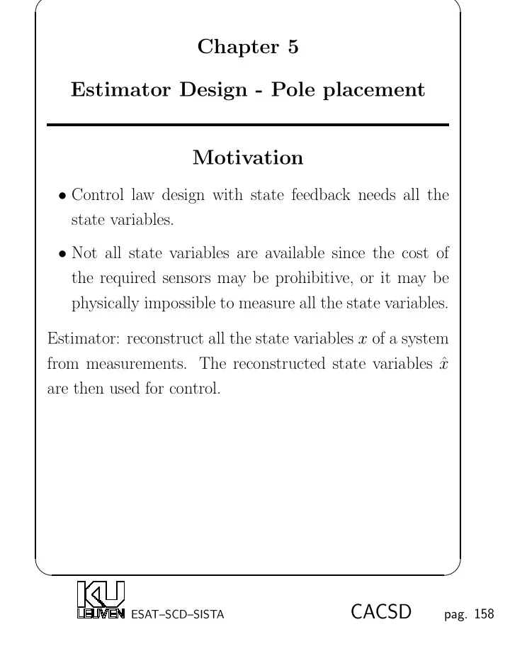
✬ ✩ Chapter 5 Estimator Design - Pole placement Motivation • Control law design with state feedback needs all the state variables. • Not all state variables are available since the cost of the required sensors may be prohibitive, or it may be physically impossible to measure all the state variables. Estimator: reconstruct all the state variables x of a system from measurements. The reconstructed state variables ˆ x are then used for control. ✫ ✪ CACSD pag. 158 ESAT–SCD–SISTA

✬ ✩ Motivation example Example Boeing 747 aircraft control In the Boeing 747 aircraft model, there are 4 states : the side-slip angle β , the yaw rate r , the roll rate p and the roll angle φ . Only the yaw rate r is measured with a gyroscope, while all other states are not measured. Challenge : Can we estimate the states β , p and φ from the measurement of r such that the state feedback control law can be implemented? What are the effects of the estimated states on the final closed loop system? ✫ ✪ CACSD pag. 159 ESAT–SCD–SISTA

✬ ✩ Full Order Estimators (Observers) Open loop estimator Estimator: Reconstruct a full order model of the plant dynamics: ˙ x = A ˆ ˆ x + Bu. x is the estimate of the state x . ˆ The dynamics of this estimator: Define the error in the estimate: ∆ ˜ = x − ˆ x x Then the dynamics of this error system are given by (sub- tracting the estimate from the state): ˙ x = A ˜ ˜ x (0) = x (0) − ˆ ˜ x (0) . x, ✫ ✪ CACSD pag. 160 ESAT–SCD–SISTA

✬ ✩ Process y u x x = Ax + Bu ˙ C ˙ x = A ˆ ˆ x + Bu x ˆ Estimator Disadvantage of the open loop estimator: • The error is converging to zero at the same rate as the natural dynamics of A (if A is stable). There is no way to influence the rate at which the state estimate converges to the true state. • The error will NOT converge if A is unstable. • If the model dynamics ( A, B, C, D ) are different from the system dynamics (due to inaccurate modeling for instance), in general, ˜ x will not converge to 0. ✫ ✪ CACSD pag. 161 ESAT–SCD–SISTA

✬ ✩ Estimator with feedback Estimator: Insert the feedback signal of the difference between the mea- sured and estimated outputs ( y − C ˆ x ) to correct the model: ˙ x = A ˆ ˆ x + Bu + L ( y − C ˆ x ) . where L is a constant matrix in R n × p . Dynamics of the estimator: The error dynamics are given as follows (by subtracting the estimate from the state): ˙ x = ( A − LC )˜ ˜ x (0) = x (0) − ˆ ˜ x (0) . x, ✫ ✪ CACSD pag. 162 ESAT–SCD–SISTA

✬ ✩ Process y u x x = Ax + Bu ˙ C + y ˜ − ˆ x ˙ ˆ x = A ˆ x + Bu + L ˜ y C ˆ y Estimator Properties: • By choosing the gain matrix L , the error dynamics of A − LC can be stable and much faster than the open loop dynamics A . • In case of inaccurate A and/or C , the error dynamics can still be stabilized and be faster ⇒ Robustness. ✫ ✪ CACSD pag. 163 ESAT–SCD–SISTA

✬ ✩ Estimator Design - Pole Placement Choose the gain matrix L such that the poles of the estimator are in desired positions. Let the desired locations be given by s = s 1 , s 2 , . . . , s n then the desired estimator characteristic equation is ∆ α e ( s ) = ( s − s 1 )( s − s 2 ) . . . ( s − s n ) Direct method Determine L by comparing coefficients of the two polyno- mials on both sides of the following equation : det ( sI − ( A − LC )) = ( s − s 1 )( s − s 2 ) . . . ( s − s n ) ✫ ✪ CACSD pag. 164 ESAT–SCD–SISTA

✬ ✩ Duality of estimation and control designs The problem to find L such that det ( sI − ( A − LC )) = ( s − s 1 )( s − s 2 ) . . . ( s − s n ) is equivalent to the problem to find K = L T such that sI − ( A T − C T K ) � � det = ( s − s 1 )( s − s 2 ) . . . ( s − s n ) which is the problem for state feedback control design. Further, the controllability matrix C of ( A, B ) is the trans- pose of the observability matrix O of ( A T , B T ). Thus we have the following duality relations: Control Estimation A T A C T B L T K O T C ✫ ✪ CACSD pag. 165 ESAT–SCD–SISTA

✬ ✩ Ackermann’s formula for SISO   0   0 L = α e ( A ) O − 1   .   . .     1 where O is the observability matrix. Sylvester equation for MIMO: Design procedure: • Pick an arbitrary matrix G ∈ R p × n . • Solve the Sylvester equation for X : A T X − X Λ = C T G   α 1 β 1 − β 1 α 1     ...   Λ = ,     λ 1     ... which has eigenvalues: α 1 ± jβ 1 , . . . , λ 1 , . . . . which are the desired poles of the estimator. • Obtain the static feedback gain L = ( GX − 1 ) T . ✫ ✪ CACSD pag. 166 ESAT–SCD–SISTA

✬ ✩ Estimator Pole Selection The dynamics of the state estimation error are governed by the eigenvalues of A − LC . Obviously, all eigenvalues are chosen to be stable. Concerning the estimator pole se- lection there is a fundamental trade-off between sensitivity of the estimation error to sensor noise and speed of con- vergence. The smaller R e { eig( A − LC ) } , the faster the estimation error goes to zero. However, for small eigenval- ues rapid changes in the signals will also introduce rapid changes in the estimation error. The estimated state will change nervously. In the next chapter we will describe an optimal solution for this dilemma which is the Kalman fil- ter. Consider a control system with process noise w and sensor noise v : x = Ax + Bu + B 1 w, ˙ y = Cx + v then the estimator error will be : ˙ x = ( A − LC )˜ ˜ x + B 1 w − Lv ✫ ✪ CACSD pag. 167 ESAT–SCD–SISTA

✬ ✩ Rules of thumb: • Trade-off between a fast dynamic response (of the esti- mator) and a good sensor noise reduction. ⇒ “large” L or “small ” L . • Trade-off between process noise reduction and sensor noise reduction. ⇒ “large” L or “small ” L . Consider the following first order system x = − x + u ˙ y = x + v where v is sensor noise. Now compare 2 estimators : A − LC = − 10 and A − LC = − 2. There is no input, but the initial state is 1. The dynamics for A − LC = − 10 are faster but more subject to noise : 1.2 − state evolution 1 −− estimated state, A−LC=−10 0.8 .. estimated state, A−LC=−2 0.6 0.4 0.2 0 −0.2 ✫ 0 0.5 1 1.5 2 2.5 3 3.5 4 4.5 5 ✪ time (s) CACSD pag. 168 ESAT–SCD–SISTA

✬ ✩ Examples of estimator design Example Boeing 747 aircraft control - Estimator design with pole placement (Ackermann’s method) We have designed a state feedback control law, and the desired closed-loop poles are at − 0 . 0051 , − 0 . 468 , − 1 . 106 , − 9 . 89 , − 0 . 279 ± 0 . 628 i. For a fast response of the estimator, we make the poles of the estimator 5 times faster than the desired closed-loop poles : − 0 . 0255 , − 2 . 34 , − 5 . 53 , − 49 . 45 , − 1 . 395 ± 3 . 14 i. The characteristic polynomial of the estimator α e ( s ) = s 6 + 60 . 14 s 5 + 575 . 4 s 4 + 2453 s 3 + 6595 s 2 + 7721 s + 192 . 6 α e ( A ) =   − 1 . 13 e + 6 0 0 0 0 0  − 4 . 48 e + 4 − 5 . 15 e + 3 − 4 . 49 e + 3 6 . 01 e + 2 2 . 24 e + 2 0      − 5 . 38 e + 5 3 . 27 e + 3 − 4 . 06 e + 3 1 . 91 e + 2 1 . 50 e + 2 0      1 . 81 e + 5 − 8 . 17 e + 3 1 . 55 e + 4 − 3 . 62 e + 3 − 6 . 12 e + 2 0      − 1 . 72 e + 4 − 1 . 45 e + 4 8 . 58 e + 3 4 . 54 e + 3 − 6 . 54 e + 1 0     5 . 38 e + 4 3 . 17 e + 3 3 . 84 e + 3 − 3 . 14 e + 1 5 . 48 e + 1 − 1 . 73 e + 3 ✫ ✪ CACSD pag. 169 ESAT–SCD–SISTA

✬ ✩ The observability matrix equals O =   0 0 1 0 0 − 3 . 33 e − 1   − 4 . 75 e + 0 5 . 98 e − 1 − 4 . 48 e − 1 − 3 . 18 e − 2 0 1 . 11 e − 1     4 . 96 e + 1 − 2 . 04 e − 1 − 4 . 46 e − 1 7 . 70 e − 2 2 . 48 e − 2 − 3 . 70 e − 2       − 4 . 94 e + 2 − 4 . 90 e − 1 2 . 50 e − 1 − 1 . 32 e − 2 − 8 . 49 e − 3 1 . 23 e − 2     4 . 94 e + 3 2 . 17 e − 1 4 . 66 e − 1 − 4 . 96 e − 2 − 2 . 03 e − 2 − 4 . 12 e − 3     − 4 . 94 e + 4 4 . 18 e − 1 − 2 . 95 e − 1 5 . 31 e − 3 9 . 01 e − 3 1 . 37 e − 3 Then the feedback gain for the estimator is   2 . 5047 e + 01   − 2 . 0517 e + 03     − 5 . 1935 e + 03   L =    − 2 . 4851 e + 04      − 4 . 0914 e + 04     − 1 . 5728 e + 04 ✫ ✪ CACSD pag. 170 ESAT–SCD–SISTA

✬ ✩ Example Tape drive control - Estimator design with pole placement (Sylvester equation) The desired estimator poles are again set to be 5 times faster than the desired closed-loop poles: − 2 . 2550 ± 4 . 6850 i, − 4 . 7350 ± 2 . 9050 i, − 5 . 8000 , − 5 . 8000 . Take an arbitrary matrix G : � � − 0 . 508 − 0 . 248 − 0 . 445 − 0 . 209 − 1 . 064 1 . 133 G = 0 . 885 − 0 . 726 − 0 . 613 0 . 562 0 . 352 0 . 150 Solve the Sylvester equation for X : A T X − X Λ e = C T G Λ e is a block diagonal matrix with the eigenvalues equal to the desired estimator poles:   − 2 . 225 4 . 685   − 4 . 685 − 2 . 225     − 4 . 735 2 . 905   Λ c = .    − 2 . 905 − 4 . 735      − 5 . 8     − 5 . 8 ✫ ✪ CACSD pag. 171 ESAT–SCD–SISTA