Chapter 2: Basics from Probability Theory and Statistics 2.1 - PowerPoint PPT Presentation

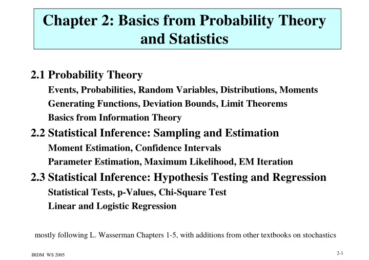
Chapter 2: Basics from Probability Theory and Statistics 2.1 Probability Theory Events, Probabilities, Random Variables, Distributions, Moments Generating Functions, Deviation Bounds, Limit Theorems Basics from Information Theory 2.2 Statistical Inference: Sampling and Estimation Moment Estimation, Confidence Intervals Parameter Estimation, Maximum Likelihood, EM Iteration 2.3 Statistical Inference: Hypothesis Testing and Regression Statistical Tests, p-Values, Chi-Square Test Linear and Logistic Regression mostly following L. Wasserman Chapters 1-5, with additions from other textbooks on stochastics 2-1 IRDM WS 2005

2.1 Basic Probability Theory A probability space is a triple ( Ω , E, P) with • a set Ω of elementary events (sample space), • a family E of subsets of Ω with Ω∈ E which is closed under ∩ , ∪ , and − with a countable number of operands (with finite Ω usually E=2 Ω ), and • a probability measure P: E → → → [0,1] with P[ Ω ]=1 and → P[ ∪ i A i ] = i P[A i ] for countably many, pairwise disjoint A i Properties of P: P[A] + P[ ¬ A] = 1 P[A ∪ B] = P[A] + P[B] – P[A ∩ B] P[ ∅ ] = 0 (null/impossible event) P[ Ω ] = 1 (true/certain event) 2-2 IRDM WS 2005

Independence and Conditional Probabilities Two events A, B of a prob. space are independent if P[A ∩ B] = P[A] P[B]. A finite set of events A={A 1 , ..., A n } is independent = ∏ if for every subset S ⊆ A the equation P[ A ] P[A ] i i holds. ∈ ∈ A S A S i i The conditional probability P[A | B] of A under the ∩ P [ A B ] condition (hypothesis) B is defined as: = P [ A | B ] P [ B ] Event A is conditionally independent of B given C if P[A | BC] = P[A | C]. 2-3 IRDM WS 2005

Total Probability and Bayes’ Theorem Total probability theorem: For a partitioning of Ω into events B 1 , ..., B n : n = P[ A] P[ A| B ] P[ B ] i i = i 1 P [ B | A ] P [ A ] = Bayes‘ theorem: P [ A | B ] P [ B ] P[A|B] is called posterior probability P[A] is called prior probability 2-4 IRDM WS 2005

Random Variables A random variable (RV) X on the prob. space ( Ω , E, P) is a function X: Ω → M with M ⊆ R s.t. {e | X(e) ≤ x} ∈ E for all x ∈ M (X is measurable). F X : M → [0,1] with F X (x) = P[X ≤ x] is the (cumulative) distribution function (cdf) of X. With countable set M the function f X : M → [0,1] with f X (x) = P[X = x] is called the (probability) density function (pdf) of X; in general f X (x) is F‘ X (x). For a random variable X with distribution function F, the inverse function F -1 (q) := inf{x | F(x) > q} for q ∈ [0,1] is called quantile function of X. (0.5 quantile (50 th percentile) is called median) Random variables with countable M are called discrete , otherwise they are called continuous . For discrete random variables the density function is also referred to as the probability mass function . 2-5 IRDM WS 2005

Important Discrete Distributions p ) − x 1 x = = − • Bernoulli distribution with parameter p: P [ X x ] p (1 ∈ for x {0,1} • Uniform distribution over {1, 2, ..., m}: 1 = = = ≤ ≤ P [ X k ] f ( k ) for 1 k m X m • Binomial distribution (coin toss n times repeated; X: #heads): n − k n k = = = − P [ X k ] f ( k ) p ( 1 p ) X k • Poisson distribution (with rate λ ): k λ − λ = = = P [ X k ] f ( k ) e X k ! • Geometric distribution (#coin tosses until first head): k = = = − P [ X k ] f ( k ) ( 1 p ) p X • 2-Poisson mixture (with a 1 +a 2 =1): k k λ λ − λ − λ = = = 1 + 2 1 2 P [ X k ] f ( k ) a e a e X 1 2 k ! k ! 2-6 IRDM WS 2005

Important Continuous Distributions • Uniform distribution in the interval [a,b] 1 = ≤ ≤ f X ( x ) for a x b ( 0 otherwise ) − b a • Exponential distribution (z.B. time until next event of a Poisson process) with rate λ = lim ∆ t → 0 (# events in ∆ t) / ∆ t : − λ x = λ ≥ f ( x ) e for x 0 ( 0 otherwise ) X − λ − λ x x = λ + − λ 1 2 f ( x ) p e ( 1 p ) e • Hyperexponential distribution: X 1 2 + a 1 a b → > f ( x ) for x b , 0 otherwise • Pareto distribution: X b x → c f ( x ) Example of a „heavy-tailed“ distribution with X α + 1 x 1 = F ( x ) • logistic distribution: X e − x + 1 2-7 IRDM WS 2005

Normal Distribution (Gaussian Distribution) • Normal distribution N( µ µ µ , σ µ σ σ σ 2 ) (Gauss distribution; 2 − µ ( x ) − approximates sums of independent, 2 σ = 1 2 f ( x ) e identically distributed random variables): X 2 πσ 2 • Distribution function of N(0,1): 2 x − z Φ = 1 2 ( z ) e dx π 2 − ∞ Theorem: Let X be normal distributed with expectation µ and variance σ 2 . − µ = X Then Y : σ is normal distributed with expectation 0 and variance 1. 2-8 IRDM WS 2005

Multidimensional (Multivariate) Distributions Let X 1 , ..., X m be random variables over the same prob. space with domains dom(X 1 ), ..., dom(X m ). The joint distribution of X 1 , ..., X m has a density function f ( x , ..., x ) X , ..., X 1 m 1 m = with ... f ( x , ..., x ) 1 X , ..., X 1 m 1 m ∈ ∈ x dom ( X ) x dom ( X ) 1 1 m m = or ... f ( x ,...,x ) dx ...dx 1 X 1,...,Xm 1 m m 1 dom( X ) dom( X ) 1 m The marginal distribution of X i in the joint distribution of X 1 , ..., X m has the density function ... ... f ( x , ..., x ) or X , ..., X 1 m 1 m − + x x x x 1 i 1 i 1 m ... ... f ( x , ..., x ) dx ... dx dx ... dx + − X , ..., X 1 m m i 1 i 1 1 1 m X X − X + X 1 i 1 i 1 m 2-9 IRDM WS 2005

� � � � Important Multivariate Distributions multinomial distribution (n trials with m-sided dice): n k k = ∧ ∧ = = = 1 m P [ X k ... X k ] f ( k , ..., k ) p ... p 1 1 m m X , ..., X 1 m m 1 1 m k ... k 1 m n n ! = with : k ... k k ! ... k ! 1 m 1 m multidimensional normal distribution: − 1 T 1 − − µ Σ − µ ( x ) ( x ) 1 = 2 f ( x ) e X , ..., X 1 m m π Σ ( 2 ) with covariance matrix Σ with Σ ij := Cov(X i ,X j ) 2-10 IRDM WS 2005

Moments For a discrete random variable X with density f X = is the expectation value (mean) of X E [ X ] k f X k ( ) ∈ k M i i = is the i-th moment of X E [ X ] k f ( k ) X ∈ k M 2 2 2 = − = − is the variance of X V [ X ] E [( X E [ X ]) ] E [ X ] E [ X ] For a continuous random variable X with density f X + ∞ = is the expectation value of X E [ X ] x f ( x ) dx X − ∞ + ∞ i i = is the i-th moment of X E [ X ] x f ( x ) dx X − ∞ 2 2 2 = − = − is the variance of X V [ X ] E [( X E [ X ]) ] E [ X ] E [ X ] + = + E [ X Y ] E [ X ] E [ Y ] Theorem: Expectation values are additive: (distributions are not) 2-11 IRDM WS 2005

Properties of Expectation and Variance E[aX+b] = aE[X]+b for constants a, b E[X 1 +X 2 +...+X n ] = E[X 1 ] + E[X 2 ] + ... + E[X n ] (i.e. expectation values are generally additive, but distributions are not!) E[X 1 +X 2 +...+X N ] = E[N] E[X] if X 1 , X 2 , ..., X N are independent and identically distributed (iid RVs) with mean E[X] and N is a stopping-time RV Var[aX+b] = a 2 Var[X] for constants a, b Var[X 1 +X 2 +...+X n ] = Var[X 1 ] + Var[X 2 ] + ... + Var[X n ] if X 1 , X 2 , ..., X n are independent RVs Var[X 1 +X 2 +...+X N ] = E[N] Var[X] + E[X] 2 Var[N] if X 1 , X 2 , ..., X N are iid RVs with mean E[X] and variance Var[X] and N is a stopping-time RV 2-12 IRDM WS 2005

Correlation of Random Variables Covariance of random variables Xi and Xj:: = − − Cov ( Xi , Xj ) : E [ ( Xi E [ Xi ]) ( Xj E [ Xj ]) ] 2 2 = = − Var ( Xi ) Cov ( Xi , Xi ) E [ X ] E [ X ] Correlation coefficient of Xi and Xj Cov ( Xi , Xj ) ρ = ( Xi , Xj ) : Var ( Xi ) Var ( Xj ) Conditional expectation of X given Y=y: x f (x | y) discrete case X|Y = = E[X | Y y] x f (x | y)dx continuous case X|Y 2-13 IRDM WS 2005

Transformations of Random Variables Consider expressions r(X,Y) over RVs such as X+Y, max(X,Y), etc. 1. For each z find A z = {(x,y) | r(x,y) ≤ z} 2. Find cdf F Z (z) = P[r(x,y) ≤ z] = z f (x, y)dx dy A X,Y 3. Find pdf f Z (z) = F‘ Z (z) Important case: sum of independent RVs (non-negative) Z = X+Y F Z (z) = P[r(x,y) ≤ z] = f (x)f (y)dx dy + ≤ x y z X Y y x − z x z = x 0 f (x)f (y) dxdy = = X Y y 0 z = − x 0 f (x)F (z x) dx = X Y or in discrete case: Convolution = F (z) f (x)f (y) + ≤ Z x y z X Y x y 2-14 IRDM WS 2005