
SLIDE 1
Channels of contagion: identifying and monitoring systemic risk Rama CONT
Center for Financial Engineering, Columbia University & Laboratoire de Probabilités, CNRS- Universite de Paris VI.
Channels of contagion: identifying and monitoring systemic risk Rama - - PowerPoint PPT Presentation
Channels of contagion: identifying and monitoring systemic risk Rama CONT Center for Financial Engineering, Columbia University & Laboratoire de Probabilits, CNRS- Universite de Paris VI. In collaboration with Hamed Amini (EPFL,
Center for Financial Engineering, Columbia University & Laboratoire de Probabilités, CNRS- Universite de Paris VI.
Rama CONT: Contagion and systemic risk in financial networks
Rama CONT: Contagion and systemic risk in financial networks
Rama CONT: Contagion and systemic risk in financial networks
Rama CONT: Contagion and systemic risk in financial networks
∙ Size= 4 billion$, Daily VaR= 400 million $ in Aug 1998. ∙ Amaranth (2001): size = 9.5 billion USD, no systemic consequence. ∙ The default of Amaranth hardly made headlines: no systemic impact. ∙ The default of LTCM threatened the stability of the US banking system → Fed intervention ∙ Reason: LTCM had many counterparties in the world banking system, with large liabilities/exposures. ∙ 1: Systemic impact is not about ’net’ size but related to exposures/ connections with other institutions. ∙ 2: a firm can have a small magnitude of losses/gains AND be a source of large systemic risk
4
Rama CONT: Contagion and systemic risk in financial networks
Rama CONT: Contagion and systemic risk in financial networks
as a network – a weighted, directed graph- whose nodes are financial institutions and whose links represents exposures and receivables.
may be modeled as contagion processes on such networks
epidemiology, stability of power grids , security of computer networks, random graph theory, percolation theory
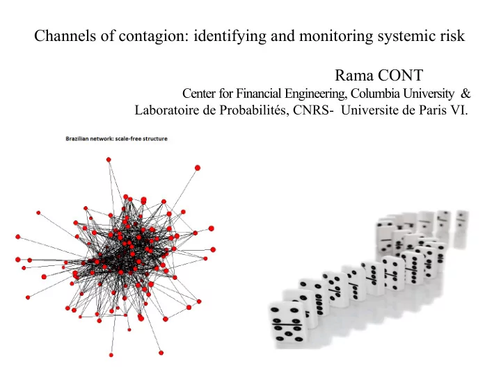
reveal a complex, heterogeneous structure which is poorly represented by simple network models used in the theoretical literature. Brazilian Interbank network (Cont, Moussa, Santos 2010)
A financial system is naturally modeled as a network of counterparty relations: a set of nodes and weighted links where ∙ nodes 푖 ∈ 푉 represent financial market participants: banks, funds, corporate borrowers/lenders, hedge funds, monolines. ∙ (directed) links represent counterparty exposures: 퐸푖푗 is the the exposure of 푖 to 푗, the maximal loss of 푖 if 푗 defaults ∙ 퐸푖푗 is understood as (positive part) of the market value of contracts of 푖 with 푗. ∙ 퐿푖푗 = 퐸푗푖 is the total liability of 푖 towards 푗. ∙ Each institution 푖 disposes of – a capital 푐푖 for absorbing market losses. Proxy for 푐푖: Tier I capital.
9
– a liquidity buffer 푙푖 Assets 퐴푖 Liabilities 퐿푖 Interbank assets Interbank liabilities ∑
푗 퐸푖푗
∑
푗 퐸푗푖
including: Liquid assets Deposits 푙0
푖
Other assets Capital 푎푖 푐푖 Table 1: Stylized balance sheet of a bank.
10
∙ Capital absorbs first losses. ∙ Default occurs if – (i) Demand for immediate payments (margin calls, derivative payouts) exceeds liquidity: 푙푖 + ∑
푗∕=푖 휋푖푗 < 0
Requires monitoring liquidity reserves and tracking potential future exposures/payouts from derivatives. – (ii) Loss due to counterparty exposure > 푐푖 ⇒ “insolvency” ⇒ lenders cut off short term funding ⇒ (i) ∙ Actual, not (Basel-type) “risk-weighted” value of exposures, assets and liabilities need to be considered.
11
Objective: quantify the losses generated across the network by the initial default of a given financial institution. Defaults can occur through
푐푖 → max(푐푖 + 휖푖, 0)
푐푗 < 퐸푗푖
available liquidity 푙푖 + ∑
푗 휋푖푗(푐 + 휖, 퐸) < 0
In cases 2 and 3 this can generate a ’domino effect’ and initiate a cascade of defaults.
30
Figure: Network structures of real-world banking systems. Austria: scale-free structure (Boss et al2004), Switzerland: sparse and centralized structure (Müller 2006).
Figure: Network structures of real-world banking systems. Hungary: multiple money center structure (Lubloy et al 2006) Brazil: scale-free structure (Cont, Bastos, Moussa 2010).
The Brazil financial system: a directed scale-free network ∙ Exposures are reportted daily to Brazilian central bank. ∙ Data set of all consolidated interbank exposures (incl. swaps)+ Tier I and Tier II capital (2007-08). ∙ 푛 ≃ 100 holdings/conglomerates, ≃ 1000 counterparty relations ∙ Average number of counterparties (degree)= 7 ∙ Heterogeneity of connectivity: in-degree (number of debtors) and out-degree (number of creditors) have heavy tailed distributions 1 푛#{푣, indeg(푣) = 푘} ∼ 퐶 푘훼푖푛 1 푛#{푣, outdeg(푣) = 푘} ∼ 퐶 푘훼표푢푡 with exponents 훼푖푛, 훼표푢푡 between 2 and 3. ∙ Heterogeneity of exposures: heavy tailed Pareto distribution with exponent between 2 and 3.
14
10 10
110
210
−310
−210
−110
In Degree Pr(K ≥ k)
α = 2.1997 kmin = 6 p−value = 0.0847
Network in June 2007
10 10
110
210
−310
−210
−110
In Degree Pr(K ≥ k)
α = 2.7068 kmin = 13 p−value = 0.2354
Network in December 2007
10 10
110
210
−310
−210
−110
In Degree Pr(K ≥ k)
α = 2.2059 kmin = 7 p−value = 0.0858
Network in March 2008
10 10
110
210
−310
−210
−110
In Degree Pr(K ≥ k)
α = 3.3611 kmin = 21 p−value = 0.7911
Network in June 2008
10 10
110
210
−310
−210
−110
In Degree Pr(K ≥ k)
α = 2.161 kmin = 6 p−value = 0.0134
Network in September 2008
10 10
110
210
−310
−210
−110
In Degree Pr(K ≥ k)
α = 2.132 kmin = 5 p−value = 0.0582
Network in November 2008
Figure 3: Brazilian financial network: distribution of in-degree.
16
0.2 0.4 0.6 0.8 1 0.1 0.2 0.3 0.4 0.5 0.6 0.7 0.8 0.9 1 p−value = 0.99998 p−value = 0.99919 p−value = 0.99998 p−value = 0.9182 p−value = 0.9182
Q−Q Plot of In Degree
Pr(K(i)≤ k) Pr(K(j)≤ k)
0.2 0.4 0.6 0.8 1 0.1 0.2 0.3 0.4 0.5 0.6 0.7 0.8 0.9 1 p−value = 0.99234 p−value = 0.99998 p−value = 0.99998 p−value = 0.99234 p−value = 0.84221
Q−Q Plot of Out Degree
Pr(K(i)≤ k) Pr(K(j)≤ k)
0.2 0.4 0.6 0.8 1 0.1 0.2 0.3 0.4 0.5 0.6 0.7 0.8 0.9 1 p−value = 0.99998 p−value = 0.9683 p−value = 0.9683 p−value = 0.99234 p−value = 0.64508
Q−Q Plot of Degree
Pr(K(i)≤ k) Pr(K(j)≤ k)
Jun/07 vs. Dec/07 Dec/07 vs. Mar/08 Mar/08 vs. Jun/08 Jun/08 vs. Sep/08 Sep/08 vs. Nov/08 45o line − (i) vs. (j) Jun/07 vs. Dec/07 Dec/07 vs. Mar/08 Mar/08 vs. Jun/08 Jun/08 vs. Sep/08 Sep/08 vs. Nov/08 45o line − (i) vs. (j) Jun/07 vs. Dec/07 Dec/07 vs. Mar/08 Mar/08 vs. Jun/08 Jun/08 vs. Sep/08 Sep/08 vs. Nov/08 45o line − (i) vs. (j)
Figure 4: Brazilian financial network: stability of degree distribu- tions across dates.
17
10
−910
−710
−510
−310
−110
110
−410
−310
−210
−110
Exposures × 10−10 in BRL Pr(X ≥ x)
α = 1.9792 xmin = 0.0039544 p−value = 0.026
Network in June 2007
10
−910
−710
−510
−310
−110
−410
−310
−210
−110
Exposures × 10−10 in BRL Pr(X ≥ x)
α = 2.2297 xmin = 0.0074042 p−value = 0.6
Network in December 2007
10
−910
−710
−510
−310
−110
−410
−310
−210
−110
Exposures × 10−10 in BRL Pr(X ≥ x)
α = 2.2383 xmin = 0.008 p−value = 0.214
Network in March 2008
10
−1010
−810
−610
−410
−210 10
−410
−310
−210
−110
Exposures × 10−10 in BRL Pr(X ≥ x)
α = 2.3778 xmin = 0.010173 p−value = 0.692
Network in June 2008
10
−1010
−810
−610
−410
−210 10
−410
−310
−210
−110
Exposures × 10−10 in BRL Pr(X ≥ x)
α = 2.2766 xmin = 0.0093382 p−value = 0.384
Network in September 2008
10
−910
−710
−510
−310
−110
110
−310
−210
−110
Exposures × 10−10 in BRL Pr(X ≥ x)
α = 2.5277 xmin = 0.033675 p−value = 0.982
Network in November 2008
Figure 6: Brazilian network: distribution of exposures in BRL.
19
Empirical studies on interbank networks by central banks: ∙ Sheldon and Maurer (1998) for Switzerland, Furfine (1999) for the US, Upper and Worms (2000) for Germany Wells (2002) for the UK, Boss, Elsinger, Summer and Thurner (2003) for Austria, Mistrulli (2007): Italy ∙ DeGryse & Nguyen : Belgium, Soramaki et al (2007): Finland examine by simulation the impact of single or multiple defaults on bank solvency in absence of other effects (e.g. market shocks). Mostly focused on payment systems (FedWire) or FedFunds exposures and report very small loss magnitudes (in % of total assets).
27
Rama CONT: Contagion and systemic risk in financial networks
threatens the stability of the financial system
basis for systemic tax, etc. The majority of previous empirical/simulation studies has systematically underestimated the magnitude of contagion effects due to the use of
market risk: i.e. scenarios where one bank fails in an isolated way while everything else remains equal. In fact most large bank defaults happen in macreconomic stress scenarios
default of most banks have little systemic impact, some have large systemic impact
instead of forward looking, no predictive power
Given an initial set 퐴 of defaults in the network, we define a sequence 퐷푘(퐴) of default events by setting 퐷0(퐴) = 퐴 and, at each iteration, identifying the set 퐷푘(퐴) of institutions which either ∙ become insolvent due to their counterparty exposures to institutions in 퐷푘−1(퐴) which have already defaulted at the previous round 푐푘
푗 = min(푐푘−1 푗
− ∑
푣∈퐷푘−1(퐴)
(1 − 푅푣)퐸푗푣, 0) (7) ∙ lack the liquidity to pay out the contingent cash flows 휋푗푣(푐푘−1, 퐸푘−1)–margin calls or derivatives payables– triggered by the previous credit/market events: 푙푗 + ∑
푣 / ∈퐷푘−1(퐴)
휋푗푣(푐푘−1, 퐸푘−1)
(8)
31
Definition 1 (Default cascade). Given the initial default of a set 퐴 of institutions in the network, the default cascade generated by 퐴 is defined as the sequence 퐷0(퐴) ⊂ 퐷1(퐴) ⊂ ⋅ ⋅ ⋅ ⊂ 퐷푛−1(퐴) where 퐷0(퐴) = 퐴 and for 푘 ≥ 1, 푐푘
푗 = min(푐푘−1 푗
− ∑
푣∈퐷푘−1(퐴)
(1 − 푅푣)퐸푗푣, 0) (9) 퐷푘(퐴) = {푗, 푐푘
푗 = 0
∑
푣 / ∈퐷푘−1(퐴)
휋푗푣(푐푘, 퐸) < 0
} The cascade ends after at most 푛 − 1 rounds: 퐷푛−1(퐴) is the set of defaults generated by the initial default of 퐴.
32
DEFAULT IMPACT of a financial institution Case of a single default:, 퐷푛−1(푖) = cascade generated by default of 푖. We define the “default impact” 퐷퐼(푖, 푐, 푙, 퐸) of 푖 as the total loss (in $) along the default cascade initiated by 푖. 퐷퐼(푖, 푐, 푙, 퐸) = ∑
푗∈퐷푛−1(푖)
(푐푗 + ∑
푣 / ∈퐷푛−1(푖)
퐸푗푣)
퐷퐼(푖, 푐, 푙, 퐸) depends -in a deterministic way- on the network structure: matrix of exposures [퐸푗푘], liquidity reserves 푙푗, capital 푐푗. 퐷퐼(푖, 푐, 푙, 퐸) is a worst-case loss estimate and does not involve estimating the default probability of 푖.
33
(Cont, Moussa, Santos 2010)
Similarly we can define the contagion index of a set 퐴 ⊂ 푉 of financial institutions: it is the expected loss to the financial systems generated by the joint default of all institutions in 퐴: 푆(퐴) = 퐸[퐷퐼(퐴, 푐 + 휖, 퐸)∣∀푖 ∈ 퐴, 푐푖 + 휖푖 ≤ 0] 푆 then defines a set function 푆 : 풫(푉 ) → ℝ which associates to each group 퐴 of institutions a number quantifying the loss inflicted to the financial system if institutions in the set 퐴 fail. The Systemic Risk Index can be viewed, from the point of view of the regulator, as a macro-level “risk measure”.
33
10
−2
10 10
−3
10
−2
10
−1
10 log(s) log(P(CI > s)), tier I+II 10
−2
10 10
−3
10
−2
10
−1
10 log(s) log(P(CI > s)), tier I 10
−2
10 10
−3
10
−2
10
−1
10 log(s) log(P(DI > s)), tier I+II 10
−2
10 10
−3
10
−2
10
−1
10 log(s) log(P(DI > s)), tier I
Jun 2007 Dec 2007 Mar 2008 Jun 2008 Sep 2008 Nov 2008Figure 9: Heterogeneity of systemic importance: distribution of de- fault impact and contagion index across institutions, Brazilian net- work, 2007-2008.
42
10
210
410
610
810
1010
1210
310
410
510
610
710
810
910
1010
11Default impact Contagion index 5 10 15 0.1 0.2 0.3 0.4 0.5 0.6 0.7 Ratio of CI to DI
Figure 10: Evidence for contagion: contagion index can be more than thirteen times the default impact for some nodes.
43
Comparison of various capital requirement policies: (a) imposing a minimum capital ratio for all institutions in the network, (b) imposing a minimum capital ratio only for the 5% most systemic institutions, (c) imposing a capital-to-exposure ratio for the 5% most systemic institutions.
The relevance of asymptotics Most financial networks are characterized by a large number of nodes: FDIC data include several thousands of financial institutions in the US. To investigate contagion in such large networks, in particular the scaling of contagion effects with size, we can embed a given network in a sequence of networks with increasing size and studying the behavior/scaling of relevant quantities (cascade size, total loss, impact of regulatory policy) when network size increases. A probabilistic approach consists in
can be considered a typical sample
convergence) of the relevant quantities in the ensemble considered as 푛 → ∞
54
Analysis of cascades in large networks We describe the topology of a large network by the joint distribution 휇푛(푗, 푘) of in/out degrees and assume that 휇푛 has a limit 휇 when graph size increases in the following sense:
in-degree 푗 and out-degree 푘 tends to 휇(푗, 푘)).
푗,푘 푗휇(푗, 푘) = ∑ 푗,푘 푘휇(푗, 푘) =: 푚 ∈ (0, ∞) (finite expectation
property);
푖=1(푑+ 푛,푖)2 + (푑− 푛,푖)2 = 푂(푛) (second moment property). 55
j,k
Resilience to contagion This leads to a condition on the network which guarantees absence of contagion: Proposition 2 (Resilience to contagion). Denote 푝(푗, 푘, 1) the proportion of contagious links ending in nodes with degree (푗, 푘). If ∑
푗,푘
푘 휇(푗, 푘) 푗 휆 푝(푗, 푘, 1) < 1 (11) then with probability → 1 as 푛 → ∞, the default of a finite set of nodes cannot trigger the default of a positive fraction of the financial network.
62
Resilience condition: ∑
푗,푘
푘 휇(푗, 푘) 푗 휆 푝(푗, 푘, 1) < 1 (12) This leads to a decentralized recipe for monitoring/regulating systemic risk: monitoring the capital adequacy of each institution with regard to its largest exposures. This result also suggests that one need not monitor/know the entire network of counterparty exposures but simply the skeleton/ subgraph of contagious links. It also suggests that the regulator can efficiently contain contagion by focusing on fragile nodes -especially those with high connectivity- and their counterparties (e.g. by imposing higher capital requirements on them to reduce 푝(푗, 푘, 1)).
63
j,k
∙ Network analysis points to the importance (for regulators) of
∙ The example of Brazil shows the feasability of collecting such data. ∙ In many countries, exposures larger than a threshold are required to be reported. Our analysis suggest that the relevant threshold should be based on a ratio of the exposure to the capital, not ∙ Derivatives exposures (in particular credit derivatives positions) should be reported in more detail (not aggregated mark-to-market value) -notional, underlying, maturity,..- to enable liquidity stress tests of scenarios where margin calls or derivative payoffs re triggered. ∙ In all countries banks and various financial institutions are
64
required already to report risk measures (VaR, etc.) on a periodical basis to the regulators. ∙ Our approach would require these risk figures to be a disaggregated across large counterparties: banks would report a figure for exposures to each large counterparty. ∙ Large financial institutions already compute such exposures on a regular basis so requiring them to be reported is not likely to cause a major technological obstacle. ∙ In principle any counterparty is relevant, not just banks. ∙ On the other hand, only the largest exposures of an institution come into play.
65
Rama CONT: Contagion and systemic risk in financial networks
default via insolvency/ illiquidity across interlinked financial institutions.
nodes (connectivity, size): simple, homogeneous/unweighted networks may provide wrong insights on systemic risk and its control.
heterogeneity, assessments of contagion risk based on cross-sectional averages do not reflect the contribution of contagion to systemic risk.
mathematical resutls about the relation between network structure and resilience to contagion for arbitrary networks, which explain results of large-scale simulations. -> (Hamed AMINI’s talk tomorrow afternoon)
most systemic institutions - are more effective for reducing systemic risk.
limits on size and concentration of exposures (as % of capital) is more important than capital ratios based on aggregate asset size.
Rama CONT: Contagion and systemic risk in financial networks