
SLIDE 1
August 9, 2017
Christopher Herzog (YITP, Stony Brook University)
Boundary T race Anomalies and Boundary Conformal Field Theory
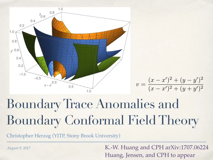
v = (x − x0)2 + (y − y0)2 (x − x0)2 + (y + y0)2
K.-W. Huang and CPH arXiv:1707.06224 Huang, Jensen, and CPH to appear