Blind (Uninformed) Search (Where we systematically explore 1. s 0 - - PDF document

1

1

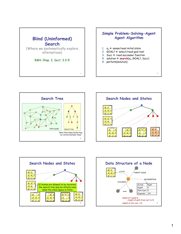
Blind (Uninformed) Search

(Where we systematically explore alternatives)

R&N: Chap. 3, Sect. 3.3–5

2

Simple Problem-Solving-Agent Agent Algorithm

1. s0 sense/read initial state 2. GOAL? select/read goal test 3. Succ read successor function 4. solution search(s0, GOAL?, Succ) 5. perform(solution)

3

Search Tree

Search tree

Note that some states may be visited multiple times

State graph

4

Search Nodes and States

1 2 3 4 5 6 7 8 1 2 3 4 5 6 7 8 1 2 3 4 5 6 7 8 1 3 5 6 8 1 3 4 5 6 7 8 2 4 7 2 1 2 3 4 5 6 7 8

5

Search Nodes and States

1 2 3 4 5 6 7 8 1 2 3 4 5 6 7 8 1 2 3 4 5 6 7 8 1 3 5 6 8 1 3 4 5 6 7 8 2 4 7 2 1 2 3 4 5 6 7 8

If states are allowed to be revisited, the search tree may be infinite even when the state space is finite If states are allowed to be revisited, the search tree may be infinite even when the state space is finite

6

Data Structure of a Node

PARENT-NODE

1 2 3 4 5 6 7 8

STATE

Depth of a node N = length of path from root to N (depth of the root = 0)

BOOKKEEPING

5 Path-Cost 5 Depth Right Action

Expanded yes

...

CHILDREN

2

7

Node expansion

The expansion of a node N of the search tree consists of: 1) Evaluating the successor function on STATE(N) 2) Generating a child of N for each state returned by the function node generation ≠ node expansion

1 2 3 4 5 6 7 8

N

1 3 5 6 8 1 3 4 5 6 7 8 2 4 7 2 1 2 3 4 5 6 7 8

8

Fringe of Search Tree

The fringe is the set of all search nodes that haven’t been expanded yet

1 2 3 4 5 6 7 8 1 2 3 4 5 6 7 8 1 2 3 4 5 6 7 8 1 3 5 6 8 1 3 4 5 6 7 8 2 4 7 2 1 2 3 4 5 6 7 8

9

Is it identical to the set of leaves?

10

Search Strategy

The fringe is the set of all search nodes that haven’t been expanded yet The fringe is implemented as a priority queue FRINGE

• INSERT(node,FRINGE)
• REMOVE(FRINGE)

The ordering of the nodes in FRINGE defines the search strategy

11

Search Algorithm #1

SEARCH#1 1. If GOAL?(initial-state) then return initial-state

• 2. INSERT(initial-node,FRINGE)
• 3. Repeat:
• a. If empty(FRINGE) then return failure
• b. N REMOVE(FRINGE)
• c. s STATE(N)
• d. For every state s’ in SUCCESSORS(s)

i. Create a new node N’ as a child of N ii. If GOAL?(s’) then return path or goal state

• iii. INSERT(N’,FRINGE)

Expansion of N

12

Performance Measures

Completeness

A search algorithm is complete if it finds a solution whenever one exists

[What about the case when no solution exists?]

Optimality

A search algorithm is optimal if it returns a minimum-cost path whenever a solution exists

Complexity

It measures the time and amount of memory required by the algorithm

3

13

Blind vs. Heuristic Strategies

Blind (or un-informed) strategies do not exploit state descriptions to order

• FRINGE. They only exploit the positions
• f the nodes in the search tree

Heuristic (or informed) strategies exploit state descriptions to order FRINGE (the most “promising” nodes are placed at the beginning of FRINGE)

14

Example

For a blind strategy, N1 and N2 are just two nodes (at some position in the search tree) Goal state N1 N2

STATE STATE

1 2 3 4 5 6 7 8 1 2 3 4 5 6 7 8 1 2 3 4 5 6 7 8

15

Example

For a heuristic strategy counting the number of misplaced tiles, N2 is more promising than N1 Goal state N1 N2

STATE STATE

1 2 3 4 5 6 7 8 1 2 3 4 5 6 7 8 1 2 3 4 5 6 7 8

16

Remark

Some search problems, such as the (n2-1)- puzzle, are NP-hard One can’t expect to solve all instances of such problems in less than exponential time (in n) One may still strive to solve each instance as efficiently as possible

This is the purpose of the search strategy

17

Blind Strategies

Breadth-first

• Bidirectional

Depth-first

• Depth-limited
• Iterative deepening

Uniform-Cost

(variant of breadth-first)

Arc cost = 1 Arc cost = c(action) ≥ ε > 0

18

Breadth-First Strategy

New nodes are inserted at the end of FRINGE

2 3 4 5 1 6 7 FRINGE = (1)

4

19

Breadth-First Strategy

New nodes are inserted at the end of FRINGE

FRINGE = (2, 3) 2 3 4 5 1 6 7

20

Breadth-First Strategy

New nodes are inserted at the end of FRINGE

FRINGE = (3, 4, 5) 2 3 4 5 1 6 7

21

Breadth-First Strategy

New nodes are inserted at the end of FRINGE

FRINGE = (4, 5, 6, 7) 2 3 4 5 1 6 7

22

Important Parameters

1) Maximum number of successors of any state branching factor b of the search tree 2) Minimal length (≠ cost) of a path between the initial and a goal state depth d of the shallowest goal node in the search tree

23

Evaluation

b: branching factor d: depth of shallowest goal node Breadth-first search is:

• Complete? Not complete?
• Optimal? Not optimal?

24

Evaluation

b: branching factor d: depth of shallowest goal node Breadth-first search is:

• Complete
• Optimal if step cost is 1

Number of nodes generated: ???

5

25

Evaluation

b: branching factor d: depth of shallowest goal node Breadth-first search is:

• Complete
• Optimal if step cost is 1

Number of nodes generated: 1 + b + b2 + … + bd = ???

26

Evaluation

b: branching factor d: depth of shallowest goal node Breadth-first search is:

• Complete
• Optimal if step cost is 1

Number of nodes generated: 1 + b + b2 + … + bd = (bd+1-1)/(b-1) = O(bd) Time and space complexity is O(bd)

27

Big O Notation

g(n) = O(f(n)) if there exist two positive constants a and N such that: for all n > N: g(n) ≤ a×f(n)

28

Time and Memory Requirements

10,000 Tbytes 3.2 years ~1014 14 100 Tbytes 11.6 days ~1012 12 1 Tbyte 2.8 hours ~1010 10 10 Gbytes 100 sec ~108 8 100 Mb 1 sec ~106 6 1 Mbyte 1 msec 11,111 4 11 Kbytes .01 msec 111 2 Memory Time # Nodes d

Assumptions: b = 10; 1,000,000 nodes/sec; 100bytes/node

29

Time and Memory Requirements

10,000 Tbytes 3.2 years ~1014 14 100 Tbytes 11.6 days ~1012 12 1 Tbyte 2.8 hours ~1010 10 10 Gbytes 100 sec ~108 8 100 Mb 1 sec ~106 6 1 Mbyte 1 msec 11,111 4 11 Kbytes .01 msec 111 2 Memory Time # Nodes d

Assumptions: b = 10; 1,000,000 nodes/sec; 100bytes/node

30

Remark

If a problem has no solution, breadth-first may run for ever (if the state space is infinite or states can be revisited arbitrary many times) 12 14 11 15 10 13 9 5 6 7 8 4 3 2 1 12 15 11 14 10 13 9 5 6 7 8 4 3 2 1

?

6

31

Bidirectional Strategy

2 fringe queues: FRINGE1 and FRINGE2

s

Time and space complexity is O(bd/2) << O(bd) if both trees have the same branching factor b Question: What happens if the branching factor is different in each direction?

32

Depth-First Strategy

New nodes are inserted at the front of FRINGE

1 2 3 4 5 FRINGE = (1)

33

Depth-First Strategy

New nodes are inserted at the front of FRINGE

1 2 3 4 5 FRINGE = (2, 3)

34

Depth-First Strategy

New nodes are inserted at the front of FRINGE

1 2 3 4 5 FRINGE = (4, 5, 3)

35

Depth-First Strategy

New nodes are inserted at the front of FRINGE

1 2 3 4 5

36

Depth-First Strategy

New nodes are inserted at the front of FRINGE

1 2 3 4 5

7

37

Depth-First Strategy

New nodes are inserted at the front of FRINGE

1 2 3 4 5

38

Depth-First Strategy

New nodes are inserted at the front of FRINGE

1 2 3 4 5

39

Depth-First Strategy

New nodes are inserted at the front of FRINGE

1 2 3 4 5

40

Depth-First Strategy

New nodes are inserted at the front of FRINGE

1 2 3 4 5

41

Depth-First Strategy

New nodes are inserted at the front of FRINGE

1 2 3 4 5

42

Depth-First Strategy

New nodes are inserted at the front of FRINGE

1 2 3 4 5

8

43

Evaluation

b: branching factor d: depth of shallowest goal node m: maximal depth of a leaf node Depth-first search is:

Complete? Optimal?

44

Evaluation

b: branching factor d: depth of shallowest goal node m: maximal depth of a leaf node Depth-first search is:

Complete only for finite search tree Not optimal

Number of nodes generated (worst case): 1 + b + b2 + … + bm = O(bm) Time complexity is O(bm) Space complexity is O(bm) [or O(m)]

[Reminder: Breadth-first requires O(bd) time and space]

45

Depth-Limited Search

Depth-first with depth cutoff k (depth at which nodes are not expanded) Three possible outcomes:

• Solution
• Failure (no solution)
• Cutoff (no solution within cutoff)

46

Iterative Deepening Search

Provides the best of both breadth-first and depth-first search Main idea: IDS For k = 0, 1, 2, … do: Perform depth-first search with depth cutoff k

(i.e., only generate nodes with depth ≤ k)

Totally horrifying !

47

Iterative Deepening

48

Iterative Deepening

9

49

Iterative Deepening

50

Performance

Iterative deepening search is:

• Complete
• Optimal if step cost =1

Time complexity is:

(d+1)(1) + db + (d-1)b2 + … + (1) bd = O(bd)

Space complexity is: O(bd) or O(d)

51

Calculation

db + (d-1)b2 + … + (1) bd = bd + 2bd-1 + 3bd-2 +… + db = (1 + 2b-1 + 3b-2 + … + db-d)×bd ≤ (Σi=1,…,∞ ib(1-i))×bd = bd (b/(b-1))2

52

d = 5 and b = 2

120 63 32 x 1 = 32 32 16 x 2 = 32 16 8 x 3 = 24 8 4 x 4 = 16 4 2 x 5 = 10 2 1 x 6 = 6 1 ID BF

120/63 ~ 2

Number of Generated Nodes

(Breadth-First & Iterative Deepening)

53

Number of Generated Nodes

(Breadth-First & Iterative Deepening) d = 5 and b = 10

123,456 111,111 100,000 100,000 20,000 10,000 3,000 1,000 400 100 50 10 6 1 ID BF

123,456/111,111 ~ 1.111

54

Comparison of Strategies

Breadth-first is complete and optimal, but has high space complexity Depth-first is space efficient, but is neither complete, nor optimal Iterative deepening is complete and

• ptimal, with the same space complexity

as depth-first and almost the same time complexity as breadth-first

Quiz: Would IDS + bi-directional search be a good combination?

10

55

Revisited States

8-queens

No

assembly planning

Few

1 2 3 4 5 6 7 8

8-puzzle and robot navigation

Many

search tree is finite search tree is infinite

56

Avoiding Revisited States

Requires comparing state descriptions Breadth-first search:

• Store all states associated with generated

nodes in VISITED

• If the state of a new node is in VISITED,

then discard the node

57

Avoiding Revisited States

Requires comparing state descriptions Breadth-first search:

• Store all states associated with generated

nodes in VISITED

• If the state of a new node is in VISITED,

then discard the node

Implemented as hash-table

• r as explicit data structure with flags

58

Avoiding Revisited States

Depth-first search:

Solution 1: – Store all states associated with nodes in current path in VISITED – If the state of a new node is in VISITED, then discard the node ??

59

Avoiding Revisited States

Depth-first search:

Solution 1: – Store all states associated with nodes in current path in VISITED – If the state of a new node is in VISITED, then discard the node Only avoids loops Solution 2: – Store all generated states in VISITED – If the state of a new node is in VISITED, then discard the node Same space complexity as breadth-first !

60

Uniform-Cost Search

Each arc has some cost c ≥ ε > 0 The cost of the path to each node N is g(N) = Σ costs of arcs The goal is to generate a solution path of minimal cost The nodes N in the queue FRINGE are sorted in increasing g(N) Need to modify search algorithm S

1

A

5

B

15

C

S G A B C

5 1 15 10 5 5

G

11

G

10

11

61

Search Algorithm #2

SEARCH#2

• 1. INSERT(initial-node,FRINGE)
• 2. Repeat:
• a. If empty(FRINGE) then return failure
• b. N REMOVE(FRINGE)
• c. s STATE(N)
• d. If GOAL?(s) then return path or goal state
• e. For every state s’ in SUCCESSORS(s)
• i. Create a node N’ as a successor of N
• ii. INSERT(N’,FRINGE)

The goal test is applied to a node when this node is expanded, not when it is generated.

62

Avoiding Revisited States in Uniform-Cost Search

For any state S, when the first node N such that

STATE(N) = S is expanded, the path to N is the

best path from the initial state to S So:

• When a node is expanded, store its state into

CLOSED

• When a new node N is generated:

– If STATE(N) is in CLOSED, discard N – If there exits a node N’ in the fringe such that

STATE(N’) = STATE(N), discard the node −− N or N’

−− with the highest-cost path