Black hole variability from limited data Simon Vaughan (Leicester) - - PowerPoint PPT Presentation

Variability from limited data Black hole variability from limited data Simon Vaughan (Leicester)

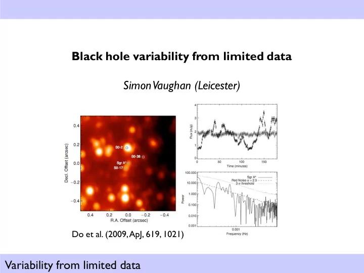
Do et al. (2009, ApJ, 619, 1021)

Variability from limited data

Outline

• 1. The periodogram (as a spectral estimator)
• 2. Problems with interpretation
• 3. In reverse: simulation from the periodogram
• 4. Few-cycle periods
• 5. Spectral analysis with short time series

a. Maximum likelihood fitting

• b. Model checking of noise spectra

c. Testing for periods

• 6. Things to watch out for
• 7. List of books, references for further reading

Variability from limited data

Spectral analysis? Y

• u‟ve been doing it for years!

Variability from limited data

The periodogram: from the DFT...

2 2 1 1

2 e.g. | ) ( | ) ( ) 1 ..., , 1 , ( ) 2 / ..., , 1 , ( / ) / 2 exp( ) 2 exp( ) ( x N t A f X A f P N k t k t N j t N j f N ijk x t if x f X

j j k j N k k N k k j k j

R I I R f X f P iI R N jk x i N jk x N jk ix N jk x f X

j j j j j j j N k k N k k N k k k j

/ tan | ) ( | ) ( ) / 2 sin( ) / 2 cos( ) / 2 sin( ) / 2 cos( ) (

1 2 2 2 1 1 1

1 1

) / 2 sin( ) / 2 cos(

N k k N k k

N jk x I N jk x R

Variability from limited data

The periodogram: from the DFT...

1 1

) / 2 sin( ) / 2 cos(

N k k N k k

N jk x I N jk x R

If xk are independent and identically (iid) distributed random variables (with a Normal distribution) – i.e. “white noise” – then Rj and Ij are also Normally

• distributed. And independent at all j (in the asymptotic limit N

). This follows from the Central Limit Theorem: the sum (or mean) of a sufficiently large number of independent random variables, each with finite mean and variance, will be approximately Normally distributed Let‟s consider a very simple case with t = 1 Expected value (mean of x) = 0 Variance (of x) =

2

Spectrum = 2

2

2 / 2 2 2 2 / 2 /

2 2 / 2 1 1 var

N j N j j N j j

N N N P N f P

Variability from limited data

The periodogram: distribution of ordinates

) / exp( 1 2 2 exp 2 1 2 / 2 ) ( exp 2 2 2 ) ( ) ( ) ( ) ( ) ( 2 exp 2 1 ~ 2 exp 2 1 ~

2 2 2 2 2 2 2 2 2 2 2 2 2 2

M P M M dP P dP rdr I R r P rdr I R rdr I prob R prob dRdI I prob R prob dp P prob I I R R

imag real r= P dr Exponential distribution of periodogram ordinates Note: does not depend on N. R I Multiplication rule

Variability from limited data

The periodogram: exponential distribution (a.k.a. chi square, 2 df) ) / exp( 1 ) ( M P M P p

Expected value (mean ) = M Variance ( 2) = M2 Std dev./mean ( / ) =100%

632 . ) 1 exp( 1 368 . ) 1 exp(

This distribution holds even when Mj is a function of j (i.e. not white)

Variability from limited data

The periodogram: exponential distribution (a.k.a. chi square, 2 df) ) 2 / exp( 2 1 ) ( X X p

Expected value (mean ) = 2 Variance ( 2) = 22 = 4 Std dev./mean ( / ) = 100% Chi-square distribution, with 2 degrees of freedom:

2 2

~ X

2 / ~

2 2 j j

M P

Gamma( /2, 2) Chi-square( ) Exponential Since R and I are independently and identically (iid) Normally distributed, the sum of squares is chi-square distributed with 2 df.

2 2 j j j

I R P

Variability from limited data

The periodogram (as a spectral estimator)

The periodogram is badly behaved (100% std. dev.) regardless of the amount of data. We say it is an inconsistent estimator of the (true) spectrum. The most popular spectral estimate (in astronomy, at least) is the averaged periodogram, where periodograms from each of M non-overlapping intervals are averaged. This is known as „Barlett‟s method‟ after M. S. Bartlett (1948, Nature, 161, 686-687)

Variability from limited data

The periodogram: Bartlett‟s method

L M M L P V L P L V Q V M M L P E L P L E Q E P L Q

j L l j L l l j L l l j j L l j j l j L l L l l j j L l l j j 2 1 2 2 1 ) ( 2 1 ) ( 1 ) ( 1 1 ) ( 1 ) (

1 1 1 ] [ 1 1 1 ] [ 1

The Bartlett averaged periodogram is a consistent spectral estimator, because the variance decreases with more data (larger L). Ideally we use independent realisations of our process, x(t), but in practice we use non-

• verlapping time segments and hope this will do (assumed ergodic).

But we are therefore limited to N/2L frequencies, with resolution L/N. We gain in variance reduction (of our estimator) but lose in frequency resolution.

Variability from limited data

Rat Electroencephalogram during Slow Wave Sleep

Examples of natural spectra

Ambient noise spectrum from a depth of 8,413 m in the Mariana Trench. A black hole

Variability from limited data

Interpreting periodograms

A message from Captain Data: “More lives have been lost looking at the raw periodogram than by any other action involving time series!” (J. Tukey 1980; quoted by D. Brillinger, 2002)

• Usually better to use log-log plots:
• log(y): more symmetric distribution of ordinates
• log(y): a natural choice for exponential distribution
• log-log: power law spectrum becomes linear
• But remember mean(log[x]) ≠ log(mean[x])
• Watch out for biases (leakage and/or aliasing)

Variability from limited data

Interpreting periodograms: aliasing

Aliasing „folds‟ power from frequencies above the Nyquist sampling frequency

• nto frequencies below the Nyquist frequency

This tends to flatten spectra at high frequencies. Greatly reduced by binning continuous data.

f t f 2 1 f t f 2 1

Variability from limited data

Interpreting periodograms: leakage

Finite duration of time series (discontinuity at ends) causes broadening or smearing of the power density. When the intrinsic spectrum is steep (e.g. ~1/f 2) this leads to a fraction of the (large) power at low frequencies leaking to higher frequencies (which have much lower intrinsic power). Hardly matters for spectra flatter than ~1/f. Can be reduced by taking longer observations (!) or tapering (yuk!)

Variability from limited data

Leakage & aliasing in sparse & finite data

Variability from limited data

In reverse: simulating noise from spectra

Variability from limited data

In reverse: simulating noise from spectra

• Davies & Harte (1987, Biometrica, 74, 95)
• Timmer & Konig (1995, A&A, 300, 707)

Now we know how the periodogram of a noise process relates to its spectrum, we can run the argument backwards, to generate a realisation of a noise process from a spectrum.

FT{C} x(t) C C Y iY X P C Y X N N j f P

j j j j j j j j j

ansform Fourier tr Inverse 5. s frequencie negative in Mirror 4. frequency) Nyquist at (set 2 / ctor complex ve a Make 3.

• n

distributi Normal standard the from and numbers random 2 /

• f

sets two generate 2. 2 / ..., , 2 , 1 at ) ( spectrum compute 1.

*

Variability from limited data

In reverse: simulating noise from spectra

• Davies & Harte (1987, Biometrica, 74, 95)
• Timmer & Konig (1995, A&A, 300, 707)

Now we know how the periodogram of a noise process relates to its spectrum, we can run the argument backwards, to generate a realisation of a noise process from a spectrum. FT{C} x(t) C C i S C N/ X P S X N/ N j f P

j j j j j j j j j j j

ansform Fourier tr Inverse 7. s frequencie negative in Mirror 6. ) exp( 2 / ctor complex ve a Make 5. frequency) Nyquist at (set ) , [

• ver

phases random 2 generate 4. m periodogra fake a get to together hese multiply t 3.

• n

distributi the from numbers random 2 generate 2. 2 / ..., , 2 , 1 at ) ( spectrum compute 1.

* 2 2

Variability from limited data

Simulation in pictures: model power spectrum

Variability from limited data

Simulation in pictures: fake periodogram (randomised power spectrum)

Variability from limited data

Simulation in pictures: random phases

Variability from limited data

Simulation in pictures: the faked complex DFT

Negative frequencies (packaged here) Real bit Imaginary bit

Variability from limited data

Simulation in pictures: inverse the DFT to get a time series

Variability from limited data

Noise simulation examples

Variability from limited data

Noise simulation examples

Variability from limited data

Noise simulation

To make realistic time series (i.e. that include aliasing and/or leakage) generate data series that are much longer than N t and/or sampled much faster than t. This is easily done in the Davies-Harte method: extrapolate power spectral model to lower/higher frequencies Where V > 1 is „oversampling‟ factor for lowest frequency, and W > 1 is „oversampling‟ factor for highest frequency. (FFTs are fast, so don‟t worry about it!) You can add other effects (e.g. realistic Poisson noise) afterwards. My advice: the best way to get a feel for how sampling affects power spectrum estimation is to simulate lots of data, with lots of different spectral shapes, and different sampling, and see how your spectrum estimates looks.

2 / ..., , 2 , 1 / VWN J J j t VN j f j

Variability from limited data

Spectral analysis with limited data: maximum likelihood (ML) fitting

Okay, we know the distribution of the periodogram, but how can we use it?

Variability from limited data

Spectral analysis with limited data: maximum likelihood (ML) fitting

Okay, we know the distribution of the periodogram, but how can we use it?

2 / 1 2 / 1

) | ( ) ( } ..., , { ) / exp( 1 ) | (

N j j j N j j j j j

M P p | p P P M P M M P p M P P

2 / 1 1

ln 2 )] ( ln[ 2 ) ( } ..., , { ) (

N j j j j G

M M P | p D M P θ θ M M

Distribution of each periodogram points Periodogram as a whole Likelihood function for periodogram (from multiplication rule – since indep.) model as a whole which is a function of G parameters The minus log likelihood (twice) = “deviance” A fit statistic: a scalar function of the G parameters for fixed data

• P. (Sometimes Whittle

likelihood.) D behaves a lot like your favourite chi-square fit statistic (e.g. minimum = best fit)

Variability from limited data

Spectral analysis with limited data: checking the noise model

How do we know if our fitted model is any good or not? Our test statistic does not have an obvious sampling (reference) distribution. Okay?... Time for some more revision... ] min[D T

Variability from limited data

• bs

T

• bs

dT H T p H T T prob p ) | ( ) | ) ( Goodness-of-fit tests

Goodness-of-fit test:

• 1. Define test statistic T(x)
• 2. Calculate observed value Tobs
• 3. calculate p=P(T

Tobs |H0) Does the model match the data? Null hypothesis H0: assumed true unless evidence to the contrary Test statistic: a scalar function of the data T(x), where x={x1, x2, …} Sampling distribution p(T | H0): probability distribution for T assuming H0 true Confidence level “p-value”: probability of

• bserving a T more extreme than

actually observed, Tobs, assuming H0 is true

Variability from limited data

Goodness-of-fit testing: interpret with care!

If p is small is rejected this does not mean The null hypothesis is true with probability p

• r

Some alternative hypothesis is true with probability 1-p but it does mean If the null hypothesis is true, the probability of such an “extreme” T is p This means that if H0 is true, we obtained some rather unlikely data. Of course, this does happen. If p is small enough, H0 will look very implausible!

Variability from limited data

Spectral analysis with limited data: checking the noise model

How do we know if our fitted model is any good or not? Our test statistic does not have an obvious sampling (reference) distribution. Okay?... Time for some more revision... ...now, the sampling distribution of the test statistic is the distribution of the T’s over the ensemble of possible „replicated‟ observations (assuming the null hypothesis H0). How do we know what this distribution looks like? Replicate some data! (Now we know how to do it.) Use Monte Carlo simulations to map out the distribution of your test statistic (such as min[D]). Can include bias (aliasing/leakage) by this method. Can account for uncertainty in the model parameters too (see Vaughan, 2010) Automatically account for number of frequencies (in period search) ] min[D T

Variability from limited data

Spectral analysis with limited data: testing for periods

Periodogram fluctuations are large, especially at low frequencies for steep spectra. These can looking like periodic signals (spectral “lines”) First thing to do is find a sensible noise spectrum.

• Fit model to periodogram
• Check the model is a reasonable fit (please!)
• Then check: plot confidence limits based on

chi-square (2 df) distribution. (Remember to account for N/2 freqs!)

] ) 1 ( 1 [ ] ln[ ] / exp[ ] / exp[ 1

/ 2 1 N X

p p p M X M X dS M S M p

Variability from limited data

Spectral analysis with limited data: testing for periods

The above does not account for uncertainties in the model, and needed explicit correction for the number of trials (frequencies). We could do the whole thing by Monte Carlo...

• Choose a sensible test statistic T (e.g. max[P/M], but could used smoothed P)
• Simulate N dataset from the null hypothesis (incl. errors on parameters)
• Map out distribution of T
• p-value = #(Tsim > Tobs) / N

And don’t restrict yourself to one test statistic. (Using the same sims!) There is often no „right‟ statistic to use, but some are more useful for diagnosing certain types of data- model misfit. Deviance (or chi-square) are „omnibus‟ tests of overall goodness-of-fit. But you could use your own that are tailored to be sensitive to the type of misfit that you are interested in... (but don‟t use lots and then quote only one!) This is the „model checking‟ approach advocated by A. Gelman et al. (see their book Bayesian Data Analysis). It expands on the idea of goodness-of-fit model „testing.‟ Remember “All models are wrong, but some are useful” (G. Box)

Variability from limited data

Spectral analysis with limited data: a worked example

time series periodogram “lowess” smoothed fitted model data/model residuals smoothed residuals

• distn. of

(smoothed data) / (best model)

• distn. of

Sum-Squared Error

Variability from limited data

Spectral analysis with limited data: multiple diagnostics

Variability from limited data

Watch out!

Just like any other situation when you are asked to assess the „significance‟ of small deviations over a noisy continuum, from a potentially large set of observations, be alert for:

• Data trawls

Finding results only in subsets of data

• Bonferroni correction

Not accounting for the number of frequencies examined

• Badly fitting continuum

What if the continuum model is wrong? (Did they check?)

• Errors on continuum?

If the model is ok, does a slight change in parameters obliterate the result?

• Publication bias

Is this just the „tip of the iceberg‟?

• Uneven sampling

Difficult to assess number of trials (frequencies searched)

• Leakage/aliasing for steep (short) and flat (under-sampled) data

All spectrum estimation is subject to bias, but its importance varies greatly with the underlying spectral form

Variability from limited data

“You know, the most amazing thing happened to me tonight. I was coming here, on the way to the lecture, and I came in through the parking lot. And you won't believe what happened. I saw a car with the license plate ARW 357. Can you imagine? Of all the millions of license plates in the state, what was the chance that I would see that particular one tonight? Amazing!”

Watch out! Post hoc reasoning

Variability from limited data

Take home message

• Take care with raw periodogram data
• If you can‟t use the Bartlett averaging, use maximum likelihood to fit the raw data
• Try “model checking” and “diagnosing misfit” rather than black-box “goodness-of-fit test”
• You can calibrate all sorts of useful diagnostics using Monte Carlo simulations – e.g.

largest data/model outlier, sum-squared error (chi-square), etc.

• Spend an afternoon playing around with simulated random time series and their

periodograms (or Bartlett averages) to understand aliasing and leakage (as well as signal-to- noise and resolution aspects) But... The power spectum is not all. In fact, it‟s a second-order statistic (spectrum). This means the power spectrum alone is enough to completely specific a stationary, Normally distributed (Gaussian), linear random process. Any deviation from this (non-Gaussian, non-stationary, non-linear) leads to higher-order effects (this information is in the phases that we threw away to make the periodogram from the DFT!).

Variability from limited data

Further reading

ISI Astrostatistics Network: http://isi.cbs.nl/COMM/AstroStat/ Priestley (1981) Spectral Analysis of Time Series – thorough, but a real brick Percival & Walden (1993) Spectral Analysis for Physical Applications van der Klis (1989) in Timing Neutron Stars Timmer & König (1995, A&A) On generating power law noise Uttley, McHardy & Papadakis (2003, MNRAS) Measuring the broad-band power spectra of AGN Uttley, McHardy & Vaughan (2005, MNRAS) Non-linear X-ray variability in X-ray binaries and AGN Vaughan (2010, MNRAS) A Bayesian test for periodic signals in red noise

Variability from limited data

A word about “three-cycle” periods

For low frequency divergent noises, most power is on scales comparable to the length

• f the entire record. But the eye is also efficient at removing a `linear' trend (because
• f perspective?), which eliminates the very longest pseudo-sinusoids.

A rule of thumb is that the strongest eye-apparent period in (actually non-periodic) data will be about

• ne-third the length of the data sample. In astronomy, one might to well to take

`three-cycle‘ quasiperiods with more than a grain of salt.

• W. Press (1978, Comments on Modern Physics, 7, 103)