Beginnings of Probability I Despite the fact that humans have played - PowerPoint PPT Presentation

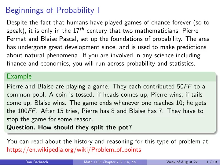
Beginnings of Probability I Despite the fact that humans have played games of chance forever (so to speak), it is only in the 17 th century that two mathematicians, Pierre Fermat and Blaise Pascal, set up the foundations of probability. The area has undergone great development since, and is used to make predictions about natural phenomena. If you are involved in any science including finance and economics, you will run across probability and statistics. Example Pierre and Blaise are playing a game. They each contributed 50 FF to a common pool. A coin is tossed. if heads comes up, Pierre wins; if tails come up, Blaise wins. The game ends whenever one reaches 10; he gets the 100 FF . After 15 tries, Pierre has 8 and Blaise has 7. They have to stop the game for some reason. Question. How should they split the pot? You can read about the history and reasoning for this type of problem at https://en.wikipedia.org/wiki/Problem of points Dan Barbasch Math 1105 Chapter 7.3, 7.4, 7.5 Week of August 27 1 / 19

PROBABILITY I Sample Space (Same as/Analogue of Universal Set) Experiment an activity/occurence with an observable result. If it repeats, call it a trial. Event Subset of a Sample Space. Mutually Exclusive Events A pair of disjoints sets, A , B such that A ∩ B = ∅ . Basic Probability. The majority of our sample spaces S are finite. We associate numbers to each event p ( A ) such that: 0 ≤ p ( A ) ≤ 1, p ( S ) = 1, If A , B are mutually exclusive, p ( A ∪ B ) = p ( A ) + p ( B ) . So if S = { a 1 , . . . , a n } it is enough to associate a number 0 ≤ p ( { a i } ) = p i ≤ 1 to each element so that the sum is equal to 1. The { p i } are called a Probability Distribution. Uniform Distribution. p i = 1 n . Dan Barbasch Math 1105 Chapter 7.3, 7.4, 7.5 Week of August 27 2 / 19

Examples YOUR TURN 2. Two fair coins are tossed. Record the outcomes and the probabilities. Fair means uniform distribution. The probabilities of each outcome is the same. S = { HH , HT , TH , TT } The probability of each s ingleton outcome is 1 4 . The probability of one head and one tail is p ( A ) = p ( { HT } ) + p ( { TH } ) = 1 4 + 1 4 = 1 A = { HT , TH } , 2 . The probability of at least one head: p ( A ) = n ( A ) n ( S ) = 3 A = { HH , HT , TH } , 4 . Dan Barbasch Math 1105 Chapter 7.3, 7.4, 7.5 Week of August 27 3 / 19

Empirical Probability I In reality we are never given the probability distribution. We guess what it is from a sample of data, and use it to make predictions about similar instances. This is called Empirical Probability in the text. It it closely related to Statistics. 57. Causes of Death. There were 2,424,059 U.S. deaths in 2007. They are listed according to cause in the following table. If a randomly selected person died in 2007, use this information to find the following probabilities. Source: Centers for Disease Control and Prevention. If a randomly selected person died in 2007, use this information to find the following probabilities. Source: Centers for Disease Control and Prevention. Dan Barbasch Math 1105 Chapter 7.3, 7.4, 7.5 Week of August 27 4 / 19

fi fi fi fi fi fi fi fi fi fi Cause Number of Deaths Heart Disease 615,651 Cancer 560,187 Cerebrovascular disease 133,990 Chronic lower respiratory disease 129,311 Accidents 117,075 Alzheimer’s disease 74,944 Diabetes mellitus 70,905 In fl uenza and pneumonia 52,847 All other causes 669,149 a. The probability that the cause of death was heart disease. b. The probability that the cause of death was cancer or heart disease. Dan Barbasch Math 1105 Chapter 7.3, 7.4, 7.5 Week of August 27 5 / 19

c. The probability that the cause of death was not an accident and was not diabetes mellitus. ANSWER . We assume uniform distribution. The sample space has size n ( S ) =615 , 651 + 560 , 187 + 133 , 990 + 129 , 311 + 117 , 075 + 74 , 944+ + 70 , 905 + 52 , 847 + 669 , 149 = 2424059 a) 615 , 651 2424095 . b) 615 , 651+560187 . 2424095 c) 2424095 − 117075 − 70905 . 2424095 Dan Barbasch Math 1105 Chapter 7.3, 7.4, 7.5 Week of August 27 6 / 19

Preliminary Questions about the Problem of Points 1 How do we set up the game in terms of the notions on the first slide? I mean sample space, event, trial ... 2 What are the assumptions about the coin toss? 3 How long will the game last? Dan Barbasch Math 1105 Chapter 7.3, 7.4, 7.5 Week of August 27 7 / 19

Answers I The sample space is { H , T } . The experiment is to toss the coin and record the outcome. { H } and { T } are mutually exclusive events. We repeat the experiment, so the whole game would be the trial. We can also set it up differently. There will be at most 19 tosses. Record all possible outcomes. That would be the sample space, and an event would be any subset. We are interested in the singletons , sets with just one element, one outcome of the game. This would be very awkward to write out. Either way, we have to associate a probability distribution. For this we need some assumtions. The following are reasonable: The coin is fair . In any one given toss, it is equally likey that heads or tails appear: p ( H ) = 1 / 2 , p ( T ) = 1 / 2 . The individual tosses are identical, and independent of each other. No outcome of a toss affects any other. Dan Barbasch Math 1105 Chapter 7.3, 7.4, 7.5 Week of August 27 8 / 19

Answers II We can now analyze the game. From 8 and 7 on, the following outcomes are possible. We record four tosses, each equally likely with probability 1 / 16 . F HHHH HHHT HHTH HTHH THHH HHTT HTHT HTTH F THHT THTH TTHH B HTTT THTT TTHT TTTH TTTT There are 11 ways F wins, 5 ways P wins. So they decide to split the pot 100 × 11 16 + 100 × 5 16 Instead of writing HHHH , we could just write HH because the game stops. But then we would assign probability 1 4 to this event. F HH HTH THH HTTH TTHH THTH 1 / 4 1 / 8 1 / 8 1 / 16 1 / 16 1 / 16 11 / 16 B HTTT TTT THTT TTHT 1 / 16 1 / 8 1 / 16 1 / 16 5 / 16 Dan Barbasch Math 1105 Chapter 7.3, 7.4, 7.5 Week of August 27 9 / 19

More Questions What is the probablity that the game will end in 1 One toss 2 Two tosses 3 Three tosses 4 Four tosses 5 Five or more tosses Dan Barbasch Math 1105 Chapter 7.3, 7.4, 7.5 Week of August 27 10 / 19

Probability Rules I Union Rule. P ( A ∪ B ) = P ( A ) + P ( B ) − P ( A ∩ B ) . Complement Rule. P ( A c ) = 1 − P ( A ) . m Odds If the odds of E occuring are m to n , then p ( E ) = m + n and n p ( E c ) = m + n . n should not be 0. Conditional Probability. P ( A | B ) = P ( A ∩ B ) P ( B ) . Careful about P ( B ) = 0 . Product Rule p ( A ∩ B ) = p ( B ) · p ( A | B ) = p ( A ) · p ( B | A ) . Independent Events. P ( A ∩ B ) = P ( A ) · P ( B ) same as P ( A | B ) = P ( A ) same as P ( B | A ) = P ( B ) . Dan Barbasch Math 1105 Chapter 7.3, 7.4, 7.5 Week of August 27 11 / 19

A standard deck of 52 cards has four suits: hearts ♥ , clubs ♣ , diamonds ♦ , and spades ♠ , with 13 cards in each suit. The hearts and diamonds are red, and the spades and clubs are black. Each suit has an ace (A), a king (K), a queen (Q), a jack (J), and cards numbered from 2 to 10. The jack, queen, and king are called face cards and for many purposes can be thought of as having values 11, 12, and 13, respectively. The ace can be thought of as the low card (value 1) or the high card (value 14). See Figure 17. We will refer to this standard deck of cards often in our discussion of probability. Dan Barbasch Math 1105 Chapter 7.3, 7.4, 7.5 Week of August 27 12 / 19

fi fi Face cards Queens Kings Jacks Aces Hearts Clubs Diamonds Spades FIGURE 17 Dan Barbasch Math 1105 Chapter 7.3, 7.4, 7.5 Week of August 27 13 / 19

� � � � � � � � � � � � � � � Conditional Probability I Banking The Midtown Bank has found that most customers at the tellers windows either cash a check or make a deposit. The following table indicates the transactions for one teller for one day. Cash Check No Check T otals Make Deposit 60 20 80 No Deposit 30 10 40 Totals 90 30 120 Letting C represent “cashing a check” and D represent “making Letting C represent cashing a check and D represent making deposit express each probability in words and find its value. 1 2 1 2 1 2 p ( D c | C ) p ( C c | D c ) p ( C | D ) 1 2 p ( C c | D ) 3 1 2 4 p (( C ∩ D ) c ) p ( C ∩ D ) Dan Barbasch Math 1105 Chapter 7.3, 7.4, 7.5 Week of August 27 14 / 19

Examples I Example (1) Two fair dice are thrown. What is the probability that a three shows or that the sum is larger than three? Example (2) A card is drawn from a well-shuffled deck. What is the probability that it is not a face card? Example (3) If the odds in favor of a horse’s winning are 4 to 6 , what is the probability that the horse will win the race? Dan Barbasch Math 1105 Chapter 7.3, 7.4, 7.5 Week of August 27 15 / 19

Examples II Example (Example 7 in Section 7.5, YOUR TURN 6) The Environmental Protection Agency is considering inspecting 6 plants for environmental compliance: 3 in Chicago, 2 in Los Angeles, and 1 in New York. Due to a lack of inspectors, they decide to inspect two plants selected at random, one this month and one next month, with each plant equally likely to be selected, but no plant selected twice. What is the probability that 1 New York plant and 1 Chicago plant are selected? Dan Barbasch Math 1105 Chapter 7.3, 7.4, 7.5 Week of August 27 16 / 19