
SLIDE 1
BBM 413 Fundamentals of Image Processing
Erkut Erdem
- Dept. of Computer Engineering
Hacettepe University
Segmentation – Part 2
Review- Image segmentation
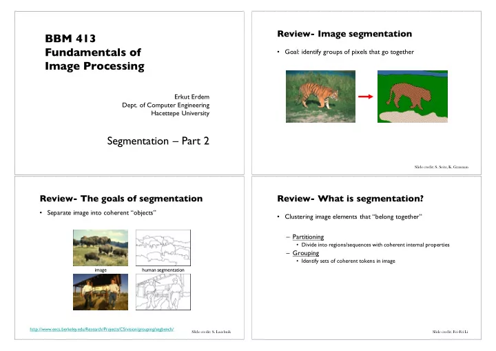
- Goal: identify groups of pixels that go together
Slide credit: S. Seitz, K. Grauman
Review- The goals of segmentation
- Separate image into coherent “objects”
http://www.eecs.berkeley.edu/Research/Projects/CS/vision/grouping/segbench/
image human segmentation
Slide credit: S. Lazebnik
Review- What is segmentation?
- Clustering image elements that “belong together”
– Partitioning
- Divide into regions/sequences with coherent internal properties
– Grouping
- Identify sets of coherent tokens in image
Slide credit: Fei-Fei Li