
SLIDE 1
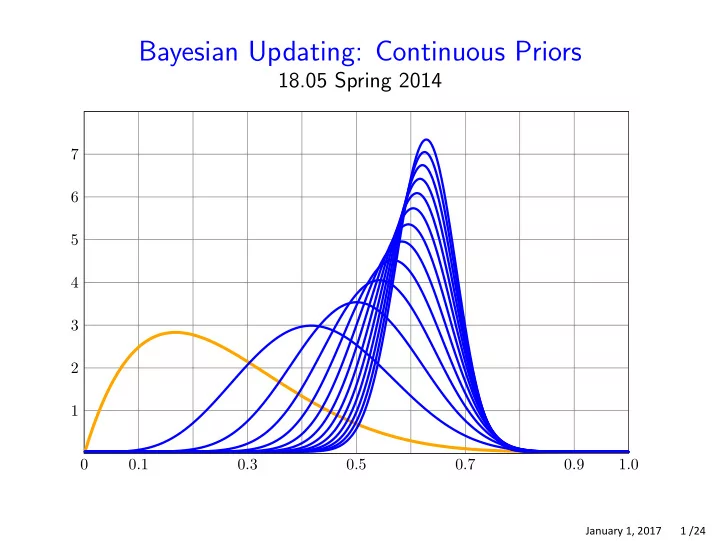
Bayesian Updating: Continuous Priors
18.05 Spring 2014
0.1 0.3 0.5 0.7 0.9 1.0 1 2 3 4 5 6 7
January 1, 2017 1 /24
Bayesian Updating: Continuous Priors 18.05 Spring 2014 7 6 5 4 3 - - PowerPoint PPT Presentation
Bayesian Updating: Continuous Priors 18.05 Spring 2014 7 6 5 4 3 2 1 0 0 . 1 0 . 3 0 . 5 0 . 7 0 . 9 1 . 0 January 1, 2017 1 /24 Continuous range of hypotheses Example. Bernoulli with unknown probability of success p . Can hypothesize
January 1, 2017 1 /24
January 1, 2017 2 /24
January 1, 2017 3 /24
January 1, 2017 4 /24
January 1, 2017 5 /24
January 1, 2017 6 /24
January 1, 2017 7 /24
January 1, 2017 8 /24
January 1, 2017 9 /24
Hypothesis H prior P (H) likelihood P (data | hyp.) Bayes numerator Posterior H P (H) (k = 0.04) P (data | hyp.) P (data | hyp.)P ( 2 H) P (data | hyp.)P (H)/P (data) 2 C k(0.01)(1-0.01) (1 − 0.01) k(0.01)(1 0. − 0.01) 0.001940921 01 2 2 C k(0.02)(1-0.02) (1 − 0.02) k(0.02)(1 02) . − 0. 0.003765396 0 02 2 C k(0.03)(1-0.03) (1 − 2 0.03) k(0.03)(1 .03 − .03) 0.005476951 C k(0.04)(1-0.04) (1 04) 0. − 2 0. k(0.04)(1 04 2 − 2 0.04) 0.007079068 C − 2 k(0.05)(1-0.05) (1 − 0.05) k(0.05)(1 0.05) 0.008575179 0.05 2 C k(0.06)(1-0.06) (1 − 2 0.06) k(0.06)(1 − 0.06) 0.009968669 0.06 2 C k(0.07)(1-0.07) (1 − 2 0.07) k(0.07)(1 0. − 0.07) 0.01126288 07 C k(0.08)(1-0.08) (1 − 2 2 0.08) k(0.08)(1 0. − 0.08) 0.01246108 08 2 2 C k(0.09)(1-0.09) (1 − 0.09) k(0.09)(1 0 09 − 0.09) 0.01356654 . 2 C k(0.1)(1-0.1) (1 − 2 0.1) k(0.1)(1 0. − .1) 0.01458243 1 2 2 C k(0.11)(1-0.11) (1 0.11) k(0.11)(1 0.11) 0.0155119 0.11 − − 2 C k(0.12)(1-0.12) (1 − 2 0.12) k(0.12)(1 − 0.12) 0.01635805 0.12 C k(0.13)(1-0.13) (1 0.13 − 2 0.13) k(0.13)(1 2 − 2 0.13) 0.01712393 2 C k(0.14)(1-0.14) (1 − 0.14) k(0.14)(1 0. − 0.14) 0.01781254 14 2 2 C k(0.15)(1-0.15) (1 − 0.15) k(0.15)(1 15) . − 0. 0.01842682 0 15 2 2 C k(0.16)(1-0.16) (1 0.16) k(0.16)(1 0.16) 0.01896969 0.16 − − C k(0.17)(1-0.17) (1 0.17 − 2 0.17) k(0.17)(1 − 2 0.17) 0.019444 − 2 − 2 C k(0.18)(1-0.18) (1 0.18) k(0.18)(1 0.18) 0.01985256 0.18 2 2 C k(0.19)(1-0.19) (1 0.19) k(0.19)(1 0.19) 0.02019812 0.19 − 2 − 2 C k(0.2)(1-0.2) (1 0.2) k(0.2)(1 0.2) 0.02048341 0.2 − − C k(0.21)(1-0.21) (1 − 2 2 0.21) k(0.21)(1 0.21 − .21) 0.02071109 2 C k(0.22)(1-0.22) (1 − 2 0.22) k(0.22)(1 − 0.22) 0.02088377 0.22 2 C k(0.23)(1-0.23) (1 − 2 0.23) k(0.23)(1 − 0.23) 0.02100402 0.23 2 2 C k(0.24)(1-0.24) (1 0.24) k(0.24)(1 0.24) 0.02107436 0.24 − − C k(0.25)(1-0.25) (1 − 2 2 0.25) k(0.25)(1 − 0.25) 0.02109727 0.25 2 2 C k(0.26)(1-0.26) (1 − 0.26) k(0.26)(1 − 0.26) 0.02107516 0.26 C 27)(1 − 2 k(0.27)(1-0.27) (1 − 2 0.27) k(0. 0.27) 0.02101042 0.27 2 2 C k(0.28)(1-0.28) (1 − 0.28) k(0.28)(1 − 0.28) 0.02090537 0.28 C k(0.29)(1-0.29) (1 0.29 − 2 0.29) k(0.29)(1 2 − 2 0.29) 0.0207623 C 3)(1 − 2 k(0.3)(1-0.3) (1 − 0.3) k(0. 0.3) 0.02058343 0.3 C k(0.31)(1-0.31) (1 0.31 − 2 0.31) k(0.31)(1 2 − 2 0.31) 0.02037095 C k(0.32)(1-0.32) (1 0.32 − 0.32) k(0.32)(1 2 − 2 0.32) 0.020127 C k(0.33)(1-0.33) (1 0.33 − 0.33) k(0.33)(1 2 − 2 0.33) 0.01985367 C 34)(1 − 2 k(0.34)(1-0.34) (1 − 0.34) k(0. 0.34) 0.01955299 0.34 C k(0.35)(1-0.35) (1 0.35 − 2 0.35) k(0.35)(1 2 − 2 0.35) 0.01922695 C − 2 k(0.36)(1-0.36) (1 − 0.36) k(0.36)(1 0.36) 0.01887751 0.36 C k(0.37)(1-0.37) (1 0.37 − 2 0.37) k(0.37)(1 2 − 2 0.37) 0.01850656 C − 2 k(0.38)(1-0.38) (1 − 0.38) k(0.38)(1 0.38) 0.01811595 0.38 C − 2 k(0.39)(1-0.39) (1 − 2 0.39) k(0.39)(1 0.39) 0.01770747 0.39 2 C k(0.4)(1-0.4) (1 − 2 0.4) k(0.4)(1 − 0.4) 0.01728288 0.4 2 C k(0.41)(1-0.41) (1 − 2 0.41) k(0.41)(1 0. − 0.41) 0.01684389 41 2 2 C k(0.42)(1-0.42) (1 − 0.42) k(0.42)(1 01639214 .42 − 0.42) 0. 2 C k(0.43)(1-0.43) (1 − 2 0.43) k(0.43)(1 0. − 0.43) 0.01592925 43 2 C k(0.44)(1-0.44) (1 − 2 0.44) k(0.44)(1 − 0.44) 0.01545678 0.44 2 C k(0.45)(1-0.45) (1 − 2 0.45) k(0.45)(1 − 0.45) 0.01497625 0.45 C k(0.46)(1-0.46) (1 0.46 − 2 0.46) k(0.46)(1 − 2 0.46) 0.0144891 2 2 C k(0.47)(1-0.47) (1 − 0.47) k(0.47)(1 0 47 − 0.47) 0.01399677 . C k(0.48)(1-0.48) (1 − 2 2 0.48) k(0.48)(1 0.48 − 0.48) 0.01350062 − 2 − 2 C k(0.49)(1-0.49) (1 0.49) k(0.49)(1 0.49) 0.01300196 0.49 C k(0.5)(1-0.5) (1 0.5 − 2 0.5) k(0.5)(1 − 2 0.5) 0.01250208 2 2 C k(0.51)(1-0.51) (1 − 0.51) k(0.51)(1 . − .51) 0.0120022 0 51 2 C k(0.52)(1-0.52) (1 − 2 0.52) k(0.52)(1 0. − .52) 0.01150349 52 2 C k(0.53)(1-0.53) (1 − 2 0.53) k(0.53)(1 − 0.53) 0.01100707 0.53 C k(0.54)(1-0.54) (1 54) 0. − 2 0. k(0.54)(1 54 − 2 0.54) 0.01051404 C k(0.55)(1-0.55) (1 − 2 2 0.55) k(0.55)(1 0 55 − 0.55) 0.01002542 . C − 2 2 k(0.56)(1-0.56) (1 0.56) k(0.56)(1 . 56 − 0.56) 0 009542198 0. 2 2 C k(0.57)(1-0.57) (1 0.57 − .57) k(0.57)(1 − 0.57) 0.009065309 2 2 C k(0.58)(1-0.58) (1 0.58) k(0.58)(1 0.58) 0.008595641 0.58 − 2 − 2 C k(0.59)(1-0.59) (1 0.59) k(0.59)(1 0.59) 0.008134034 0.59 − 2 − 2 C k(0.6)(1-0.6) (1 − 0.6) k(0.6)(1 − 0.6) 0.00768128 0.6 C − 2 k(0.61)(1-0.61) (1 − 2 0.61) k(0.61)(1 0.61) 0.007238124 0.61 2 C k(0.62)(1-0.62) (1 − 2 0.62) k(0.62)(1 − 0.62) 0.006805262 0.62 2 2 C k(0.63)(1-0.63) (1 − 0.63) k(0.63)(1 0. − 0.63) 0.006383342 63 2 2 C k(0.64)(1-0.64) (1 − 0.64) k(0.64)(1 005972963 .64 − 0.64) 0. 2 C k(0.65)(1-0.65) (1 − 2 0.65) k(0.65)(1 0. − .65) 0.005574679 65 2 2 C k(0.66)(1-0.66) (1 0.66) k(0.66)(1 0.66) 0.005188993 0.66 − − C0.67 k(0.67)(1-0.67) (1 − 0.67)2 k(0.67)(1 − 0.67)2 0.004816361 C0.68 k(0.68)(1-0.68) (1 − 0.68)2 k(0.68)(1 − 0.68)2 0.004457191 C0.69 k(0.69)(1-0.69) (1 − 0.69)2 k(0.69)(1 − 0.69)2 0.004111843
January 1, 2017 10 / 23
January 1, 2017 11 /24
January 1, 2017 12 /24
x f(x) c d P(c ≤ X ≤ d) x f(x) x dx probability f(x)dx
January 1, 2017 13 /24
January 1, 2017 14 /24
January 1, 2017 15 /24
January 1, 2017 16 /24
January 1, 2017 17 /24
January 1, 2017 18 /24
January 1, 2017 19 /24
January 1, 2017 20 /24
January 1, 2017 21 /24
January 1, 2017 22 /24
January 1, 2017 23 /24
MIT OpenCourseWare https://ocw.mit.edu
Spring 2014 For information about citing these materials or our Terms of Use, visit: https://ocw.mit.edu/terms.