
SLIDE 1
Bayesian Updating: Discrete Priors: 18.05 Spring 2014
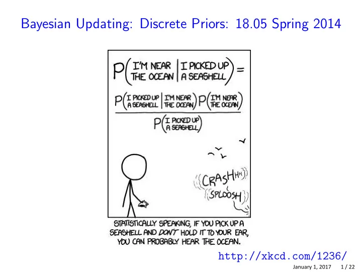
http://xkcd.com/1236/
January 1, 2017 1 / 22
Bayesian Updating: Discrete Priors: 18.05 Spring 2014 - - PowerPoint PPT Presentation
Bayesian Updating: Discrete Priors: 18.05 Spring 2014 http://xkcd.com/1236/ January 1, 2017 1 / 22 Learning from experience Which treatment would you choose? 1. Treatment 1: cured 100% of patients in a trial. 2. Treatment 2: cured 95% of
January 1, 2017 1 / 22
January 1, 2017 2 / 22
January 1, 2017 3 / 22
1 Represent this information with a tree and use Bayes’ theorem to
2 3 4
January 1, 2017 4 / 22
January 1, 2017 5 / 22
January 1, 2017 6 / 22
January 1, 2017 7 / 22
January 1, 2017 8 / 22
January 1, 2017 9 / 22
January 1, 2017 10 / 22
January 1, 2017 11 / 22
January 1, 2017 12 / 22
January 1, 2017 13 / 22
January 1, 2017 14 / 22
January 1, 2017 15 / 22
January 1, 2017 16 / 22
January 1, 2017 17 / 22
January 1, 2017 18 / 22
January 1, 2017 19 / 22
January 1, 2017 20 / 22
January 1, 2017 21 / 22
MIT OpenCourseWare https://ocw.mit.edu
Spring 2014 For information about citing these materials or our Terms of Use, visit: https://ocw.mit.edu/terms.