
SLIDE 1
1
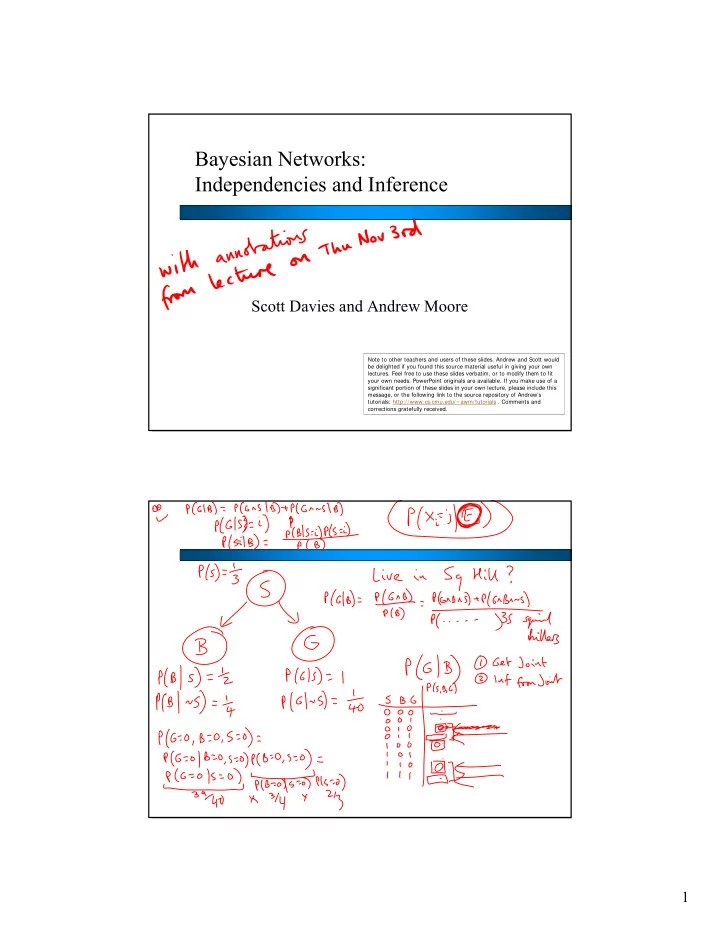
Bayesian Networks: Independencies and Inference
Scott Davies and Andrew Moore
Note to other teachers and users of these slides. Andrew and Scott would be delighted if you found this source material useful in giving your own
- lectures. Feel free to use these slides verbatim, or to modify them to fit
your own needs. PowerPoint originals are available. If you make use of a significant portion of these slides in your own lecture, please include this message, or the following link to the source repository of Andrew’s tutorials: http://www.cs.cmu.edu/~ awm/tutorials . Comments and corrections gratefully received.