Association Rules from transactional databases ! Mining multilevel - PDF document

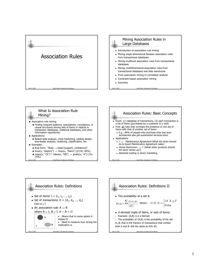
Mining Association Rules in Large Databases ! Introduction to association rule mining ! Mining single-dimensional Boolean association rules Association Rules from transactional databases ! Mining multilevel association rules from transactional databases ! Mining multidimensional association rules from transactional databases and data warehouse ! From association mining to correlation analysis ! Constraint-based association mining ! Summary May 23, 2001 Data Mining: Concepts and Techniques 1 May 23, 2001 Data Mining: Concepts and Techniques 2 What Is Association Rule Association Rules: Basic Concepts Mining? ! Given: (1) database of transactions, (2) each transaction is ! Association rule mining: a list of items (purchased by a customer in a visit) ! Finding frequent patterns, associations, correlations, or ! Find: all rules that correlate the presence of one set of causal structures among sets of items or objects in items with that of another set of items transaction databases, relational databases, and other information repositories. ! E.g., 98% of people who purchase tires and auto accessories also get automotive services done ! Applications: ! Applications ! Basket data analysis, cross-marketing, catalog design, loss-leader analysis, clustering, classification, etc. ! ? ⇒ Maintenance Agreement (What the store should do to boost Maintenance Agreement sales) ! Examples: ! Home Electronics ⇒ ? (What other products should ! Rule form: “Body → Η ead [support, confidence]”. the store stocks up?) ! buys(x, “diapers”) → buys(x, “beers”) [0.5%, 60%] ! Attached mailing in direct marketing ! major(x, “CS”) ^ takes(x, “DB”) → grade(x, “A”) [1%, 75%] May 23, 2001 Data Mining: Concepts and Techniques 3 May 23, 2001 Data Mining: Concepts and Techniques 4 Association Rules: Definitions Association Rules: Definitions II ! Set of items : I = {i 1 , i 2 , …, i m } ! The probability of a set A: ! Set of transactions : D = {d 1 , d 2 , …, d n } ∑  1 if ⊆ X Y C ( A , d ) i Where:  C ( X , Y ) = Each d i ⊆ I ( ) = i P A  0 else | D | ! An association rule : A ⇒ B where A ⊂ I, B ⊂ I, A ∩ B = ∅ ! k-itemset : tuple of items, or sets of items: Example: {A,B} is a 2-itemset • Means that to some extent A • A implies B. The probability of {A,B} is the probability of the set • • Need to measure how strong the A ∪ B, that is the fraction of transactions that contain B implication is. I both A and B. Not the same as P(A ∩ B). May 23, 2001 Data Mining: Concepts and Techniques 5 May 23, 2001 Data Mining: Concepts and Techniques 6 1

Rule Measures: Support and Association Rules: Definitions III Confidence Customer ! Find all the rules X ⇒ Y given buys both thresholds for minimum confidence ! Support of a rule A ⇒ B is the probability of the and minimum support. itemset {A,B}. This gives an idea of how often ! support, s , probability that a the rule is relevant. transaction contains {X, Y} Y: ! confidence, c, conditional ! support(A ⇒ B ) = P({A,B}) Customer X: Customer probability that a transaction buys diaper buys beer ! Confidence of a rule A ⇒ B is the conditional having X also contains Y probability of B given A. This gives a measure With minimum support 50%, Transaction ID Items Bought and minimum confidence of how accurate the rule is. 2000 A,B,C 50%, we have 1000 A,C ! confidence(A ⇒ B) = P(B|A) ! A ⇒ C (50%, 66.6%) 4000 A,D = support({A,B}) / support(A) ! C ⇒ A (50%, 100%) 5000 B,E,F May 23, 2001 Data Mining: Concepts and Techniques 7 May 23, 2001 Data Mining: Concepts and Techniques 8 Chapter 6: Mining Association Association Rule Mining: A Road Map Rules in Large Databases ! Boolean vs. quantitative associations (Based on the types of values ! Association rule mining handled) ! Mining single-dimensional Boolean association rules ! buys(x, “SQLServer”) ^ buys(x, “DMBook”) → buys(x, “DBMiner”) [0.2%, 60%] from transactional databases ! age(x, “30..39”) ^ income(x, “42..48K”) → buys(x, “PC”) [1%, 75%] ! Mining multilevel association rules from transactional ! Single dimension vs. multiple dimensional associations (see ex. Above) databases ! Single level vs. multiple-level analysis ! Mining multidimensional association rules from ! What brands of beers are associated with what brands of diapers? transactional databases and data warehouse ! Various extensions and analysis ! Correlation, causality analysis ! From association mining to correlation analysis ! Association does not necessarily imply correlation or causality ! Constraint-based association mining ! Maxpatterns and closed itemsets ! Summary ! Constraints enforced ! E.g., small sales (sum < 100) trigger big buys (sum > 1,000)? May 23, 2001 Data Mining: Concepts and Techniques 9 May 23, 2001 Data Mining: Concepts and Techniques 10 Mining Frequent Itemsets: the Mining Association Rules—An Example Key Step Transaction ID Items Bought ! Find the frequent itemsets : the sets of items that have Min. support 50% 2000 A,B,C at least a given minimum support Min. confidence 50% 1000 A,C ! A subset of a frequent itemset must also be a Frequent Itemset Support 4000 A,D frequent itemset {A} 75% 5000 B,E,F {B} 50% ! i.e., if { A, B } is a frequent itemset, both { A } and { B } {C} 50% should be a frequent itemset For rule A ⇒ C : {A,C} 50% ! Iteratively find frequent itemsets with cardinality support = support({ A, C }) = 50% from 1 to k (k- itemset ) confidence = support({ A, C })/support({ A }) = 66.6% ! Use the frequent itemsets to generate association The Apriori principle: rules. Any subset of a frequent itemset must be frequent May 23, 2001 Data Mining: Concepts and Techniques 11 May 23, 2001 Data Mining: Concepts and Techniques 12 2

The Apriori Algorithm The Apriori Algorithm — Example Database D ! Join Step: C k is generated by joining L k-1 with itself itemset sup. itemset sup. L 1 C 1 TID Items {1} 2 ! Prune Step: Any (k-1)-itemset that is not frequent cannot be {1} 2 100 1 3 4 {2} 3 a subset of a frequent k-itemset {2} 3 Scan D 200 2 3 5 {3} 3 ! Pseudo-code: {3} 3 300 1 2 3 5 {4} 1 C k : Candidate itemset of size k {5} 3 400 2 5 {5} 3 L k : frequent itemset of size k C 2 itemset C 2 itemset sup L 1 = {frequent items} {1 2} L 2 itemset sup Scan D {1 2} 1 for ( k = 1; L k != ∅ ; k ++) do begin {1 3} {1 3} 2 C k+1 = candidates generated from L k {1 3} 2 {1 5} for each transaction t in database do {1 5} 1 {2 3} 2 increment the count of all candidates in C k+1 {2 3} {2 3} 2 {2 5} 3 that are contained in t {2 5} {2 5} 3 {3 5} 2 L k+1 = candidates in C k+1 with min_support {3 5} {3 5} 2 end return ∪ k L k ; C 3 itemset L 3 itemset sup Scan D {2 3 5} {2 3 5} 2 May 23, 2001 Data Mining: Concepts and Techniques 13 May 23, 2001 Data Mining: Concepts and Techniques 14 How to Count Supports of How to do Generate Candidates? Candidates? ! Suppose the items in L k-1 are listed in an order ! Why counting supports of candidates a problem? ! Step 1: self-joining L k-1 ! The total number of candidates can be very huge insert into C k One transaction may contain many candidates ! select p.item 1 , p.item 2 , …, p.item k-1 , q.item k-1 ! Method: from L k-1 p, L k-1 q ! Candidate itemsets are stored in a hash-tree where p.item 1 =q.item 1 , …, p.item k-2 =q.item k-2 , p.item k-1 < ! Leaf node of hash-tree contains a list of itemsets q.item k-1 and counts ! Step 2: pruning ! Interior node contains a hash table forall itemsets c in C k do ! Subset function : finds all the candidates contained in forall (k-1)-subsets s of c do a transaction if (s is not in L k-1 ) then delete c from C k May 23, 2001 Data Mining: Concepts and Techniques 15 May 23, 2001 Data Mining: Concepts and Techniques 16 Methods to Improve Apriori’s Efficiency Example of Generating Candidates Hash-based itemset counting: A k -itemset whose corresponding ! ! L 3 = { abc, abd, acd, ace, bcd } hashing bucket count is below the threshold cannot be frequent ! Self-joining: L 3 *L 3 Transaction reduction: A transaction that does not contain any ! frequent k-itemset is useless in subsequent scans ! abcd from abc and abd Partitioning: Any itemset that is potentially frequent in DB must be ! ! acde from acd and ace frequent in at least one of the partitions of DB ! Pruning: Sampling: mining on a subset of given data, lower support ! threshold + a method to determine the completeness ! acde is removed because ade is not in L 3 Dynamic itemset counting: add new candidate itemsets only when ! ! C 4 ={ abcd } all of their subsets are estimated to be frequent May 23, 2001 Data Mining: Concepts and Techniques 17 May 23, 2001 Data Mining: Concepts and Techniques 18 3