Bayesian Networks 1 Recap of last lecture Probability: precise - - PDF document

Artificial Intelligence 15-381 Mar 27, 2007

Bayesian Networks 1

Michael S. Lewicki Carnegie Mellon AI: Bayes Nets 1

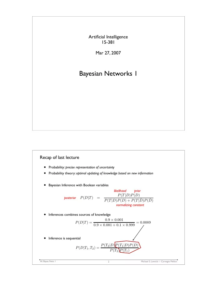
Recap of last lecture

• Probability: precise representation of uncertainty
• Probability theory: optimal updating of knowledge based on new information
• Bayesian Inference with Boolean variables
• Inferences combines sources of knowledge
• Inference is sequential

2

posterior likelihood prior normalizing constant

P(D|T ) = P(T |D)P(D) P(T |D)P(D) + P(T | ¯ D)P( ¯ D) P(D|T ) = 0.9 × 0.001 0.9 × 0.001 + 0.1 × 0.999 = 0.0089 P(D|T1, T2) = P(T2|D)P(T1|D)P(D) P(T2)P(T1)

Michael S. Lewicki Carnegie Mellon AI: Bayes Nets 1

Bayesian inference with continuous variables (recap)

3

p(θ|y, n) = p(y|θ, n)p(θ|n) p(y|n)

posterior likelihood prior normalizing constant

=

• p(y|θ, n)p(θ|n)dθ

0.1 0.2 0.3 0.4 0.5 0.6 0.7 0.8 0.9 1 ! p(! | y=1, n=5)

1 2 3 4 5 6 y p(y|!=0.05, n=5) 1 2 3 4 5 6 y p(y|!=0.2, n=5) 1 2 3 4 5 6 y p(y|!=0.35, n=5) 1 2 3 4 5 6 y p(y|!=0.5, n=5) 0.1 0.2 0.3 0.4 0.5 0.6 0.7 0.8 0.9 1 ! p(! | y=0, n=0)

prior (uniform) likelihood (Binomial) posterior (beta)

p(θ|y, n) ∝ n y

• θy(1 − θ)n−y

Michael S. Lewicki Carnegie Mellon AI: Bayes Nets 1

Today: Inference with more complex dependencies

4

• How do we represent (model) more complex probabilistic relationships?
• How do we use these models to draw inferences?

Michael S. Lewicki Carnegie Mellon AI: Bayes Nets 1

Probabilistic reasoning

5

• Suppose we go to my house and see that the door is open.
• What’s the cause? Is it a burglar? Should we go in? Call the police?
• Then again, it could just be my wife. Maybe she came home early.
• How should we represent these relationships?

Michael S. Lewicki Carnegie Mellon AI: Bayes Nets 1

Belief networks

6

• pen door

burglar wife

• In Belief networks, causal relationships are represented in directed acyclic graphs.
• Arrows indicate causal relationships between the nodes.

Michael S. Lewicki Carnegie Mellon AI: Bayes Nets 1

• How do we represent these relationships?

Types of probabilistic relationships

Direct cause

A B

Indirect cause

A B C

Common cause Common effect

A B C A B C

P(B|A) P(B|A) P(C|B) C is independent

• f A given B

P(B|A) P(C|A) P(C|A,B) Are A and B independent? Are B and C independent?

Michael S. Lewicki Carnegie Mellon AI: Bayes Nets 1

Belief networks

8

• pen door

burglar wife

• In Belief networks, causal relationships are represented in directed acyclic graphs.
• Arrows indicate causal relationships between the nodes.

How can we determine what is happening before we go in? We need more information. What else can we observe?

Michael S. Lewicki Carnegie Mellon AI: Bayes Nets 1

Explaining away

9

• pen door

burglar wife car in garage

• Suppose we notice that the car is in the garage.
• Now we infer that it’s probably my wife, and not a burglar.
• This fact “explains away” the hypothesis of a burglar.

Note that there is no direct causal link between “burglar” and “car in garage”. Yet, seeing the car changes our beliefs about the burglar.

Michael S. Lewicki Carnegie Mellon AI: Bayes Nets 1

Explaining away

10

• pen door

damaged door burglar wife car in garage

• Suppose we notice that the car is in the garage.
• Now we infer that it’s probably my wife, and not a burglar.
• This fact “explains away” the hypothesis of a burglar.
• We could also notice the door was damaged, in which case

we reach the opposite conclusion. How do we make this inference process more precise? Let’s start by writing down the conditional probabilities.

Michael S. Lewicki Carnegie Mellon AI: Bayes Nets 1

Defining the belief network

11

• pen door

damaged door burglar wife car in garage

• Each link in the graph represents a conditional relationship between nodes.
• To compute the inference, we must specify the conditional probabilities.

Michael S. Lewicki Carnegie Mellon AI: Bayes Nets 1

Defining the belief network

12

• Each link in the graph represents a conditional relationship between nodes.
• To compute the inference, we must specify the conditional probabilities.
• Let’s start with the open door. What do we specify?
• pen door

damaged door burglar wife car in garage

W B P(O|W,B) F F 0.01 F T 0.25 T F 0.05 T T 0.75

Check: Does this column have to sum to one? No! Only the full joint distribution

• does. This is a

conditional distribution. What else do we need to specify? The priors probabilities. But note that: P(¬O|W,B) = 1- P(O|W,B)

Michael S. Lewicki Carnegie Mellon AI: Bayes Nets 1

Defining the belief network

13

• Each link in the graph represents a conditional relationship between nodes.
• To compute the inference, we must specify the conditional probabilities.
• Let’s start with the open door. What do we specify?

W B P(O|W,B) F F 0.01 F T 0.25 T F 0.05 T T 0.75 P(W) 0.05

What else do we need to specify? The priors probabilities.

• pen door

damaged door burglar wife car in garage

Michael S. Lewicki Carnegie Mellon AI: Bayes Nets 1

Defining the belief network

14

• Each link in the graph represents a conditional relationship between nodes.
• To compute the inference, we must specify the conditional probabilities.
• Let’s start with the open door. What do we specify?

W B P(O|W,B) F F 0.01 F T 0.25 T F 0.05 T T 0.75 P(B) 0.001 P(W) 0.05

What else do we need to specify? The priors probabilities.

• pen door

damaged door burglar wife car in garage

Michael S. Lewicki Carnegie Mellon AI: Bayes Nets 1

Defining the belief network

15

• Each link in the graph represents a conditional relationship between nodes.
• To compute the inference, we must specify the conditional probabilities.
• Let’s start with the open door. What do we specify?

W B P(O|W,B) F F 0.01 F T 0.25 T F 0.05 T T 0.75 P(B) 0.001 P(W) 0.05 W P(C|W) F 0.01 T 0.95

Finally, we specify the remaining conditionals

• pen door

damaged door burglar wife car in garage

Michael S. Lewicki Carnegie Mellon AI: Bayes Nets 1

Defining the belief network

16

• Each link in the graph represents a conditional relationship between nodes.
• To compute the inference, we must specify the conditional probabilities.
• Let’s start with the open door. What do we specify?

W B P(O|W,B) F F 0.01 F T 0.25 T F 0.05 T T 0.75 P(B) 0.001 P(W) 0.05 B P(D|B) F 0.001 T 0.5

• pen door

damaged door burglar wife car in garage

W P(C|W) F 0.01 T 0.95

Finally, we specify the remaining conditionals Now what?

Michael S. Lewicki Carnegie Mellon AI: Bayes Nets 1

Calculating probabilities using the joint distribution

17

• What the probability that the door is open, it is my wife and not a burglar, we see the

car in the garage, and the door is not damaged?

• Mathematically, we want to compute the expression: P(o,w,¬b,c,¬d) = ?
• We can just repeatedly apply the rule relating joint and conditional probabilities.
• P(x,y) = P(x|y) P(y)

Michael S. Lewicki Carnegie Mellon AI: Bayes Nets 1

• pen door

damaged door burglar wife car in garage

Calculating probabilities using the joint distribution

18

• The probability that the door is open, it is my wife and not a burglar, we see the car in

the garage, and the door is not damaged.

• P(o,w,¬b,c,¬d) = P(o|w,¬b,c,¬d)P(w,¬b,c,¬d)

= P(o|w,¬b)P(w,¬b,c,¬d) = P(o|w,¬b)P(c|w,¬b,¬d)P(w,¬b,¬d) = P(o|w,¬b)P(c|w)P(w,¬b,¬d) = P(o|w,¬b)P(c|w)P(¬d|w,¬b)P(w,¬b) = P(o|w,¬b)P(c|w)P(¬d|¬b)P(w,¬b) = P(o|w,¬b)P(c|w)P(¬d|¬b)P(w)P(¬b)

Michael S. Lewicki Carnegie Mellon AI: Bayes Nets 1

• pen door

damaged door burglar wife car in garage

Calculating probabilities using the joint distribution

19

• P(o,w,¬b,c,¬d) = P(o|w,¬b)P(c|w)P(¬d|¬b)P(w)P(¬b)

= 0.05 0.95 0.999 0.05 0.999 = 0.0024

• This is essentially the probability that my wife is home and leaves the door open.

W B P(O|W,B) F F 0.01 F T 0.25 T F 0.05 T T 0.75 P(B) 0.001 P(W) 0.05 B P(D|B) F 0.001 T 0.5 W P(C|W) F 0.01 T 0.95

Michael S. Lewicki Carnegie Mellon AI: Bayes Nets 1

Calculating probabilities in a general Bayesian belief network

20

• Note that by specifying all the conditional probabilities, we have also specified the joint
• probability. For the directed graph above:

P(A,B,C,D,E) = P(A) P(B|C) P(C|A) P(D|C,E) P(E|A,C)

• The general expression is:

P(x1, . . . , xn) ≡ P(X1 = x1 ∧ . . . ∧ Xn = xn) =

n

• i=1

P(xi|parents(Xi))

With this we can calculate (in principle) the probability of any joint probability.

C E A B D

This implies that we can also calculate any conditional probability.

Michael S. Lewicki Carnegie Mellon AI: Bayes Nets 1

Calculating conditional probabilities

21

• Using the joint we can compute any conditional probability too
• The conditional probability of any one subset of variables given another disjoint subset is

where p ∈ S is shorthand for all the entries of the joint matching subset S.

• How many terms are in this sum?

P(S1|S2) = P(S1 ∧ S2) P(S2) = p ∈ S1 ∧ S2 p ∈ S2 2N

The number of terms in the sums is exponential in the number of variables. In fact, general querying Bayes nets is NP complete.

Michael S. Lewicki Carnegie Mellon AI: Bayes Nets 1

So what do we do?

• There are also many approximations:
• stochastic (MCMC) approximations
• approximations
• The are special cases of Bayes nets for which there are fast, exact algorithms:
• variable elimination
• belief propagation

22

Michael S. Lewicki Carnegie Mellon AI: Bayes Nets 1

Belief networks with multiple causes

• In the models above, we specified the

joint conditional density by hand.

• This specified the probability of a

variable given each possible value of the causal nodes.

• Can this be specified in a more generic

way?

• Can we avoid having to specify every

entry in the joint conditional pdf?

• For this we need to specify:

P(X | parents(X))

• One classic example of this function is

the “Noisy-OR” model.

23

• pen door

burglar wife

W B P(O|W,B) F F 0.01 F T 0.25 T F 0.05 T T 0.75

Michael S. Lewicki Carnegie Mellon AI: Bayes Nets 1

Defining causal relationships using Noisy-OR

• We assume each cause Cj can produce

effect Ei with probability fij.

• The noisy-OR model assumes the parent

causes of effect Ei contribute independently.

• The probability that none of them

caused effect Ei is simply the product of the probabilities that each one did not cause Ei.

• The probability that any of them caused

Ei is just one minus the above, i.e.

24

P(Ei|par(Ei)) = P(Ei|C1, . . . , Cn) = 1 −

• i

(1 − P(Ei|Cj)) = 1 −

• i

(1 − fij) catch cold (C) touch contaminated

• bject (O)

hit by viral droplet (D) fCD fCO eat contaminated food (F) fCF 1 − (1 − fCD)(1 − fCO)(1 − fCF ) P(C|D, O, F) =

• Could either model causes and

effects

• Or equivalently stochastic

binary features.

• Each input xi encodes the

probability that the ith binary input feature is present.

• The set of features

represented by j is defined by weights fij which encode the probability that feature i is an instance of j.

A general one-layer causal network

Each column is a distinct eight-dimensional binary feature.

The data: a set of stochastic binary patterns

There are five underlying causal feature patterns. What are they?

Each column is a distinct eight-dimensional binary feature. true hidden causes of the data

The data: a set of stochastic binary patterns

This is a learning problem, which we’ll cover in later lecture.

Michael S. Lewicki Carnegie Mellon AI: Bayes Nets 1

Hierarchical Statistical Models

A Bayesian belief network:

pa(Si) Si D

The joint probability of binary states is P(S|W) =

• i

P(Si|pa(Si), W) The probability Si depends only on its parents: P(Si|pa(Si), W) =

• h(

j Sjwji)

if Si = 1 1 − h(

j Sjwji)

if Si = 0 The function h specifies how causes are combined, h(u) = 1 − exp(−u), u > 0. Main points:

• hierarchical structure allows model to form

high order representations

• upper states are priors for lower states
• weights encode higher order features

28

Michael S. Lewicki Carnegie Mellon AI: Bayes Nets 1 29

Next time

• Inference methods in Bayes Nets
• Example with continuous variables
• More general types of probabilistic networks