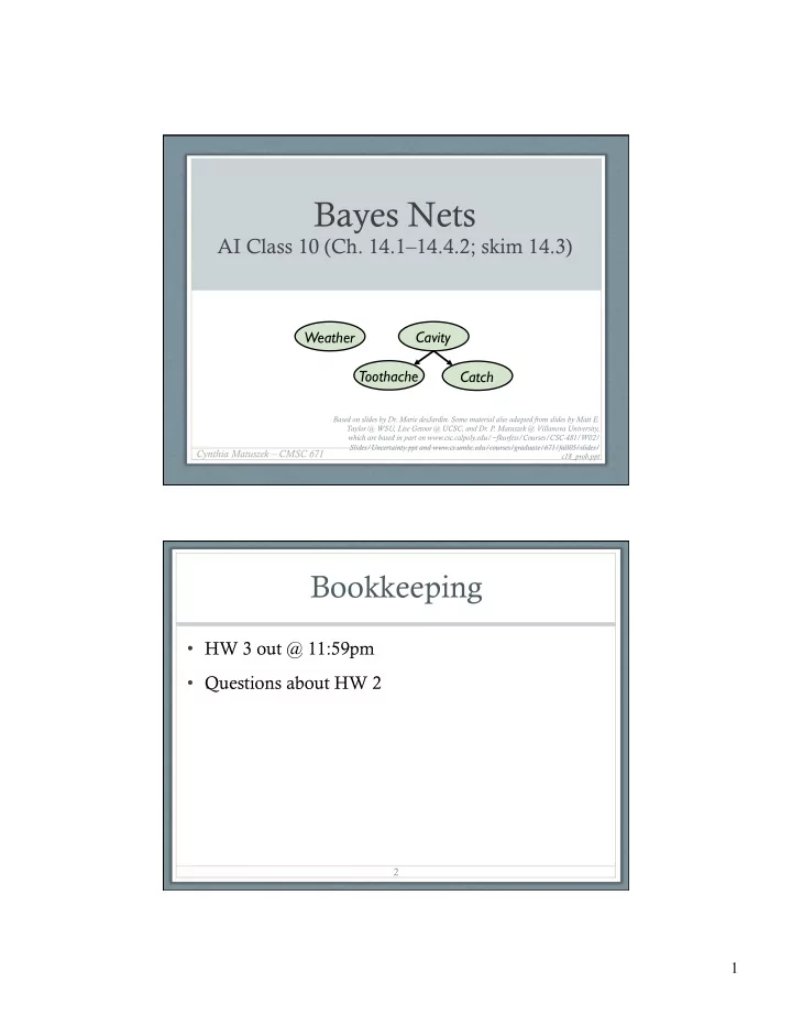
Bayes Nets AI Class 10 (Ch. 14.114.4.2; skim 14.3) Weather Cavity - PDF document

Bayes Nets AI Class 10 (Ch. 14.1–14.4.2; skim 14.3) Weather Cavity Toothache Catch Based on slides by Dr. Marie desJardin. Some material also adapted from slides by Matt E. Taylor @ WSU, Lise Getoor @ UCSC, and Dr. P. Matuszek @ Villanova University, which are based in part on www.csc.calpoly.edu/~fkurfess/Courses/CSC-481/W02/ Slides/Uncertainty.ppt and www.cs.umbc.edu/courses/graduate/671/fall05/slides/ Cynthia Matuszek – CMSC 671 c18_prob.ppt Bookkeeping • HW 3 out @ 11:59pm • Questions about HW 2 2 1

Today’s Class • Bayesian networks • Network structure • Conditional probability tables • Conditional independence • Inference in Bayesian networks • Exact inference • Approximate inference 3 Review: Independence What does it mean for A and B to be independent ? • P(A) ⫫ P(B) • A and B do not affect each other’s probability • P ( A ∧ B ) = P ( A ) P ( B ) 4 2

Review: Conditioning What does it mean for A and B to be conditionally independent given C? • A and B don’t affect each other if C is known • P (A ∧ B | C) = P (A | C) P (B | C) 6 Review: Bayes’ Rule What is Bayes’ Rule ? P ( H i | E j ) = P ( E j | H i ) P ( H i ) P ( E j ) What’s it useful for? • Diagnosis: effect is perceived, want to know cause P ( cause | effect ) = P ( effect | cause ) P ( cause ) P ( effect ) R&N, 495–496 8 3

Review: Joint Probability What is the joint probability of A and B? • P (A,B) • The probability of any pair of legal assignments. • Generalizing to > 2, of course • Booleans: expressed as a matrix/table A B alarm ¬ alarm T T 0.09 ≍ T F 0.1 burglary 0.09 0.01 F T 0.01 ¬ burglary 0.1 0.8 F F 0.8 • Continuous domains: probability functions 9 Bayes’ Nets: Big Picture • Problems with full joint distribution tables as our probabilistic models: • Joint gets way too big to represent explicitly • Unless there are only a few variables • Hard to learn (estimate) anything empirically about more than a few variables at a time • Why? A ¬A E ¬E E ¬E B 0.01 0.08 0.001 0.009 ¬B 0.01 0.09 0.01 0.79 10 Slides derived from Matt E. Taylor, WSU 4

Bayes’ Nets: Big Picture • Bayes’ nets: a technique for describing complex joint distributions (models) using simple, local distributions (conditional probabilities) • A type of graphical models • We describe how variables interact locally • Local interactions chain together to give global, indirect interactions Weather Cavity Toothache Catch 11 Slides derived from Matt E. Taylor, WSU Example: Insurance 12 Slides derived from Matt E. Taylor, WSU 5

Example: Car 13 Slides derived from Matt E. Taylor, WSU Graphical Model Notation • Nodes: variables (with domains) • Can be assigned (observed) or unassigned (unobserved) • Arcs: interactions • Indicate “direct influence” between • Formally: encode conditional independence • For now: imagine that Weather Cavity arrows mean causation Toothache • (in general, they don’t!) Catch 14 Slides derived from Matt E. Taylor, WSU 6

Bayesian Belief Networks (BNs) • Let’s formalize the semantics of a BN • A set of nodes, one per variable X • An arc between each con-influential node • A directed, acyclic graph • A conditional distribution for each node • A collection of distributions over X • One for each combination of parents’ values P ( X | A 1 … A n ) • CPT: conditional probability table • Description of a noisy “causal” process 15 Slides derived from Matt E. Taylor, WSU Bayesian Belief Networks (BNs) • Definition: BN = (DAG, CPD) • DAG : directed acyclic graph (BN’s structure ) • Nodes : random variables • Typically binary or discrete • Methods exist for continuous variables • Arcs : indicate probabilistic dependencies between nodes • Lack of link signifies conditional independence • CPD : conditional probability distribution (BN’s parameters ) • Conditional probabilities at each node, usually stored as a table (conditional probability table, or CPT ) 16 7

Bayesian Belief Networks (BNs) • Definition: BN = (DAG, CPD) • DAG : directed acyclic graph (BN’s structure ) • CPD : conditional probability distribution (BN’s parameters ) • Conditional probabilities at each node, usually stored as a table (conditional probability table, or CPT ) P ( x i | π i ) where π i is the set of all parent nodes of x i • Root nodes are a special case • No parents, so use priors in CPD: π i = ∅ , so P ( x i | π i ) = P ( x i ) 17 Example BN P(A) = 0.001 a P(C|A) = 0.2 P(B|A) = 0.3 P(C| ¬ A) = 0.005 b c P(B| ¬ A) = 0.001 d e P(D|B,C) = 0.1 P(E|C) = 0.4 P(D|B, ¬ C) = 0.01 P(E| ¬ C) = 0.002 P(D| ¬ B,C) = 0.01 P(D| ¬ B, ¬ C) = 0.00001 We only specify P(A) etc., not P(¬A), since they have to sum to one 18 8

Probabilities in BNs • Bayes’ nets implicitly encode joint distributions as a product of local conditional distributions . • To see probability of a full assignment , multiply all the relevant conditionals together: n ∏ P ( x 1 , x 2 ,... x n ) = P ( x i | parents ( X i ) ) Cavity i = 1 • Example: Toothache Catch P (+cavity, +catch, ¬toothache) = ? • This lets us reconstruct any entry of the full joint 19 Slides derived from Matt E. Taylor, WSU Conditional Independence and Chaining • Conditional independence assumption: P ( x i | π i , q ) = P ( x i | π i ) • q is any set of variables (nodes) other than x i and its successors π i q • π i blocks influence of other nodes on x i and its successors x i • That is, q influences x i only through variables in π i ) • With this assumption, complete joint probability distribution of all variables in the network can be represented by (recovered from) local CPDs by chaining these CPDs: n P ( x i | π i ) P ( x 1 ,..., x n ) = Π i = 1 20 9

The Chain Rule n P ( x i | π i ) P ( x 1 ,..., x n ) = Π i = 1 e.g, P ( x 1 ,..., x n ) = P ( x 1 ) P ( x 2 | x 1 ) P ( x 3 | x 1 , x 2)... • Decomposition: P (Traffic, Rain, Umbrella) = � P (Rain) P (Traffic | Rain) P (Umbrella | Rain, Traffic) • With assumption of conditional independence: P (Traffic, Rain, Umbrella) = � P (Rain) P (Traffic | Rain) P (Umbrella | Rain) • Bayes’ nets express conditional independence assumptions 21 Slides derived from Matt E. Taylor, WSU Chaining: Example a b c d e Computing the joint probability for all variables is easy: P(a, b, c, d, e) = P(e | a, b, c , d) P(a, b, c, d) by the product rule = P(e | c) P(a, b, c, d) by cond. indep. assumption = P(e | c) P(d | a, b, c ) P(a, b, c) = P(e | c) P(d | b, c) P(c | a, b) P(a, b) = P(e | c) P(d | b, c) P(c | a) P(b | a) P(a) 22 10

Topological Semantics • A node is conditionally independent of its non- descendants given its parents • A node is conditionally independent of all other nodes in the network given its parents, children, and children’s parents (also known as its Markov blanket ) • The method called d-separation can be applied to decide whether a set of nodes X is independent of another set Y, given a third set Z 23 Independence and Causal Chains • Important question about a BN: • Are two nodes independent given certain evidence? • If yes, can prove using algebra (tedious in general) • If no, can prove with a counter example • Question: are X and Z necessarily independent? • No. (E.g., low pressure causes rain, which causes traffic) • X can influence Z, Z can influence X (via Y) • This configuration is a “causal chain” 24 Slides derived from Matt E. Taylor, WSU 11

Two More Main Patterns • Common Cause: • Y cause X and Y causes Z • Are X and Z independent? • Are X and Z independent given Y? • Common Effect: • Two causes of one effect • Are X and Z independent? (yes) • Are X and Z independent given Y? → No ! • Observing an effect “ activates ” influence between possible causes. 25 Slides derived from Matt E. Taylor, WSU Inference in Bayesian Networks Chapter 14.4.1-14.4.2 Some material borrowed from Lise Getoor 27 12

Inference Tasks • Simple queries: Compute posterior marginal P(X i | E=e) • E.g., P(NoGas | Gauge=empty, Lights=on, Starts=false) • Conjunctive queries: • P(X i , X j | E=e) = P(X i | e=e) P(X j | X i , E=e) • Optimal decisions: • Decision networks include utility information • Probabilistic inference gives P(outcome | action, evidence) • Value of information: Which evidence should we seek next? • Sensitivity analysis: Which probability values are most critical? • Explanation: Why do I need a new starter motor? 28 Approaches to Inference • Exact inference • Approximate inference • Stochastic simulation / • Enumeration sampling methods • Belief propagation in polytrees • Markov chain Monte Carlo methods • Variable elimination • Genetic algorithms • Clustering / join tree algorithms • Neural networks • Simulated annealing • Mean field theory 29 13