Basic Terminology REVIEW from Data Structures! G = ( V , E ); V is - - PDF document

Basic Terminology

REVIEW from Data Structures! G = (V , E); V is set of n nodes, E is set of m edges Node or Vertex: a point in a graph Edge: connection between nodes Weight: numerical cost or length of an edge Direction: arrow on an edge Path: sequence (u0, u1, . . . , uk) with every (ui−1, ui) ∈ E Cycle: path that starts and ends at the same node

CS 355 (USNA) Unit 6 Spring 2012 1 / 48

Examples

Roads and intersections People and relationships Computers in a network Web pages and hyperlinks Makefile dependencies Scheduling tasks and constraints (many more!)

CS 355 (USNA) Unit 6 Spring 2012 2 / 48

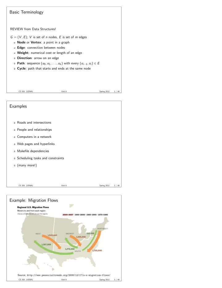
Example: Migration Flows

Source: http://www.pewsocialtrends.org/2008/12/17/u-s-migration-flows/

CS 355 (USNA) Unit 6 Spring 2012 3 / 48

Graph Representations

Adjacency Matrix: n × n matrix of weights. A[i][j] has the weight of edge (ui, uj). Weights of non-existent edges usually 0 or ∞. Size: Adjacency Lists: Array of n lists; each list has node-weight pairs for the *outgoing edges* of that node. Size: Implicit: Adjacency lists computed on-demand. Can be used for infinite graphs! Unweighted graphs have all weights either 0 or 1. Undirected graphs have every edge in both directions.

CS 355 (USNA) Unit 6 Spring 2012 4 / 48

Simple Example

Adjacency Matrix: a b c d e a b c d e Adjacency List:

CS 355 (USNA) Unit 6 Spring 2012 5 / 48

Search Template

search(G)

1

colors := size -n array

• f

"white"s

2

fringe := new collection

3

// initialize fringe with node-weight pairs

4

while fringe not empty do

5

(u,w1) := fringe.top()

6

i f colors[u] = "white" then

7

colors[u] := "gray"

8

f o r each

• utgoing

edge (u,v,w2)

• f

u do

9

fringe.update(v,w1+w2)

10

end f o r

11

e l s e i f colors[u] = "gray" then

12

colors[u] := "black"

13

fringe.remove(u,w1)

14

end i f

15

end while

CS 355 (USNA) Unit 6 Spring 2012 6 / 48

Basic Searches

To find a path from u to v, initialize fringe with (u, 0), and exit when we color v to “gray”. Two choices: Depth-First Search fringe is a stack. Updates are pushes. Breadth-First Search fringe is a queue. Updates are enqueues.

CS 355 (USNA) Unit 6 Spring 2012 7 / 48

DAGs

Some graphs are acyclic by nature. An acyclic undirected graph is a. . . DAGs (Directed Acyclic Graphs) are more interesting: Can have more than n − 1 edges Always at least one “source” and at least one “sink” Examples:

CS 355 (USNA) Unit 6 Spring 2012 8 / 48

Linearization

Problem

Input: A DAG G = (V , E) Output: Ordering of the n vertices in V as (u1, u2, . . . , un) such that only “forward edges” exist, i.e., for all (ui, uj) ∈ E), i < j. (Also called “topological sort”.) Applications:

CS 355 (USNA) Unit 6 Spring 2012 9 / 48

linearize(G)

1

• rder := empty

list

2

colors := size -n array

• f

"white"s

3

fringe := new stack

4

add every node in V to fringe

5

while fringe not empty do

6

(u,w1) := fringe.top()

7

i f colors[u] = "white" then

8

colors[u] := "gray"

9

f o r each

• utgoing

edge (u,v,w2)

• f

u do

10

fringe.push(v,w2)

11

end f o r

12

e l s e i f colors[u] = "gray" then

13

colors[u] := "black"

14

• rder := u, order

15

fringe.remove(u,w1)

16

end i f

17

end while

CS 355 (USNA) Unit 6 Spring 2012 10 / 48

Linearization Example

CS 355 (USNA) Unit 6 Spring 2012 11 / 48 CS 355 (USNA) Unit 6 Spring 2012 12 / 48

Properties of DFS

Every vertex in the stack is a child of the first gray vertex below it. Every descendant of u is a child of u or a descendant of a child of u. In a DAG, when a node is colored gray its children are all white or black. In a DAG, every descendant of a black node is black.

CS 355 (USNA) Unit 6 Spring 2012 13 / 48

Dijkstra’s Algorithm

Dijkstra’s is a modification of BFS to find shortest paths. Solves the single source shortest paths problem. Used millions of times every day (!) for packet routing Main idea: Use a minimum priority queue for the fringe Requires all edge weights to be non-negative

CS 355 (USNA) Unit 6 Spring 2012 14 / 48

dijkstra(G,u)

1

colors := size -n array

• f

"white"s

2

fringe := new minimum priority queue

3

f o r each v in V do

4

add (v, infinity) to fringe

5

fringe.update(u, 0)

6

while fringe not empty do

7

(u,w1) := fringe.removeMin ()

8

colors[u] := "black"

9

print (u,w1)

10

f o r each edge (u,v,w2) with colors[v]="white" do

11

fringe.update(v,w1+w2)

12

end f o r

13

end while

Differences from the search template

fringe is a priority queue fringe is initialized with every node Updates are done to existing fringe elements No gray nodes! (No post-processing necessary.) Useful variants: Keep track of the actual paths as well as path lengths Stop when a destination vertex is found

CS 355 (USNA) Unit 6 Spring 2012 16 / 48

Dijkstra example

a b 6 c 6 d 3 2 e 4 5 1 4

CS 355 (USNA) Unit 6 Spring 2012 17 / 48

Dijkstra Implementation Options

Heap Unsorted Array

• Adj. Matrix
• Adj. List

mmmmmmmmm

CS 355 (USNA) Unit 6 Spring 2012 18 / 48

Optimization Problems

An optimization problem is one where there are many solutions, and we have to find the “best” one. Examples we have seen: Optimal solution can often be made as a series of “moves” (Moves can be parts of the answer, or general decisions)

CS 355 (USNA) Unit 6 Spring 2012 19 / 48

Greedy Design Paradigm

A greedy algorithm solves an optimization problem by a sequence of “greedy moves”. Greedy moves: Are based on “local” information Don’t require “looking ahead” Should be fast to compute! Might not lead to optimal solutions Example: Counting change

CS 355 (USNA) Unit 6 Spring 2012 20 / 48

Appointment Scheduling

Problem

Given n requests for EI appointments, each with start and end time, how to schedule the maximum number of appointments? For example: Name Start End Billy 8:30 9:00 Susan 9:00 10:00 Brenda 8:00 8:20 Aaron 8:55 9:05 Paul 8:15 8:45 Brad 7:55 9:45 Pam 9:00 9:30

CS 355 (USNA) Unit 6 Spring 2012 21 / 48

Greedy Scheduling Options

How should the greedy choice be made?

1 First come, first served 2 Shortest time first 3 Earliest finish first

Which one will lead to optimal solutions?

CS 355 (USNA) Unit 6 Spring 2012 22 / 48

Proving Greedy Strategy is Optimal

Two things to prove:

1 Greedy choice is always part of an optimal solution 2 Rest of optimal solution can be found recursively CS 355 (USNA) Unit 6 Spring 2012 23 / 48

Matchings

Pairing up people or resources is a common task. We can model this task with graphs:

Maximum Matching Problem

Given an undirected, unweighted graph G = (V , E), find a subset of edges M ⊆ E such that: Every vertex touches at most one edge in M The size of M is as large as possible Greedy Algorithm: Repeatedly choose any edge that goes between two unpaired vertices and add it to M.

CS 355 (USNA) Unit 6 Spring 2012 24 / 48

Greedy matching example

l h m d i a b e c f j k g

CS 355 (USNA) Unit 6 Spring 2012 25 / 48

Maximum matching example

l h m d i a b e c f j k g

CS 355 (USNA) Unit 6 Spring 2012 26 / 48

How good is the greedy solution?

Theorem: The optimal solution is at most times the size of one produced by the greedy algorithm. Proof:

CS 355 (USNA) Unit 6 Spring 2012 27 / 48

Spanning Trees

A spanning tree in a graph is a connected subset of edges that touches every vertex. Dijkstra’s algorithm creates a kind of spanning tree. This tree is created by greedily choosing the “closest” vertex at each step. We are often interested in a minimal spanning tree instead.

CS 355 (USNA) Unit 6 Spring 2012 28 / 48

MST Algorithms

There are two greedy algorithms for finding MSTs: Prim’s. Start with a single vertex, and grow the tree by choosing the least-weight fringe edge. Identical to Dijkstra’s with different weights in the “update” step. Kruskal’s. Start with every vertex (a forest of trees) and combine trees by using the lease-weight edge between them.

CS 355 (USNA) Unit 6 Spring 2012 29 / 48

MST Examples

Prim’s:

a b 6 c 6 d 3 2 e 4 5 1 4

Kruskal’s:

a b 6 c 6 d 3 2 e 4 5 1 4

CS 355 (USNA) Unit 6 Spring 2012 30 / 48

All-Pairs Shortest Paths

Let’s look at a new problem:

Problem: All-Pairs Shortest Paths

Input: A graph G = (V , E), weighted, and possibly directed. Output: Shortest path between every pair of vertices in V Many applications in the precomputation/query model:

CS 355 (USNA) Unit 6 Spring 2012 31 / 48

Repeated Dijkstra’s

First idea: Run Dijkstra’s algortihm from every vertex. Cost: Sparse graphs: Dense graphs:

CS 355 (USNA) Unit 6 Spring 2012 32 / 48

Storing Paths

Na¨ ıve cost to store all paths: Memory wall Better way:

CS 355 (USNA) Unit 6 Spring 2012 33 / 48

a b 6 c 6 d 3 2 e 4 5 1 4

a b c d e a b c d e

Recursive Approach

Idea for a simple recursive algortihm: New parameter k: The highest-index vertex visited in any shortest path. Basic idea: Path either contains k, or it doesn’t. Three things needed:

1 Base case: k = −1. Shortest paths are just single edges. 2 Recursive step: Use basic idea above.

Compare shortest path containing k to shortest path without k.

3 Termination: When k = n, we’re done. CS 355 (USNA) Unit 6 Spring 2012 35 / 48

Recursive Shortest Paths

rshort(A,i,j,k)

Input: Adjacency matrix A and indices i, j, k Output: Shortest path from i to j that only goes through vertices 0–k

1

i f k = -1 then

2

return A[i,j]

3

e l s e

4

• ption1 := rshort(A,i,j,k-1)

5

• ption2 := rshort(A,i,k,k-1) + rshort(A,k,j,k-1)

6

return min(option1 , option2)

7

end i f

Analysis:

CS 355 (USNA) Unit 6 Spring 2012 36 / 48

Dynamic Programming Solution

Key idea: Keep overwriting shortest paths, using the same memory

FloydWarshall(A)

Input: Adjacency matrix A Output: Shortest path lengths between every pair of vertices

1

L = copy(A)

2

f o r k from 0 to n do

3

f o r i from 0 to n-1 do

4

f o r j from 0 to n-1 do

5

L[i,j] := min (L[i,j], L[i,k] + L[k,j])

6

end f o r

7

end f o r

8

end f o r

9

return L

CS 355 (USNA) Unit 6 Spring 2012 37 / 48

a c 1 f 6 d 6 e 5 4 b 1 1 2 2

a b c d e f a b c d e f

Analysis of Floyd-Warshall

Time: Space: Advantages:

CS 355 (USNA) Unit 6 Spring 2012 39 / 48

Another Dynamic Solution

What if k is the greatest number of edges in each shortest path? Let Lk be the matrix of shortest-path lengths with at most k edges. Base case: k = 1, then L1 = A, the adjacency matrix itself! Recursive step: Shortest (k + 1)-edge path is the minimum of k-edge paths, plus a single extra edge. Termination: Every path has length at most n − 1. So Ln−1 is the final answer.

CS 355 (USNA) Unit 6 Spring 2012 40 / 48

Min-Plus Arithmetic

Update step: Lk+1[i, j] = min

0≤ℓ<n(Lk[i, ℓ] + A[ℓ, j])

Min-Plus Algebra The + operation becomes “min” The · operation becomes “plus” Update step becomes:

CS 355 (USNA) Unit 6 Spring 2012 41 / 48

APSP with Min-Plus Matrix Multiplication

We want to compute An−1. Initial idea: Multiply n − 1 times. Improvement: Further improvement?

CS 355 (USNA) Unit 6 Spring 2012 42 / 48

Transitive Closure

Examples of reachability questions: Is there any way out of a maze? Is there a flight plan from one airport another? Can you tell me a is greater than b without a direct comparison? Precomputation/query formulation: Same graph, many reachability questions.

Transitive Closure Problem

Input: A graph G = (V , E), unweighted, possibly directed Output: Whether u is reachable from v, for every u, v ∈ V

CS 355 (USNA) Unit 6 Spring 2012 43 / 48

TC with APSP

One vertex is reachable from another if the shortest path isn’t infinite. Therefore transitive closure can be solved with repeated Dijkstra’s or Floyd-Warshall. Cost will be Θ(n3). Why might we be able to beat this?

CS 355 (USNA) Unit 6 Spring 2012 44 / 48

Back to Algebra

Define Tk as the reachability matrix using at most k edges in a path. What is T0? What is T1? Formula to compute Tk+1: Therefore transitive closure is just:

CS 355 (USNA) Unit 6 Spring 2012 45 / 48

The most amazing connection

(Pay attention. Minds will be blown in 3. . . 2. . . 1. . . )

CS 355 (USNA) Unit 6 Spring 2012 46 / 48

Vertex Cover

Problem: Find the smallest set of vertices that touches every edge.

l h m d i a b e c f j k g

CS 355 (USNA) Unit 6 Spring 2012 47 / 48

Approximating VC

Approximation algorithm for minimal vertex cover:

1 Find a greedy maximal matching 2 Take both vertices in every edge in the matching

Why is this always a vertex cover? How good is the approximation?

CS 355 (USNA) Unit 6 Spring 2012 48 / 48