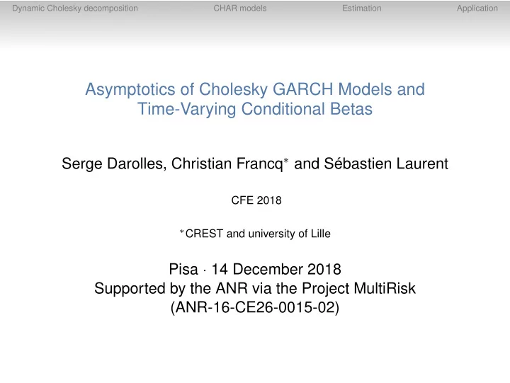
Asymptotics of Cholesky GARCH Models and Time-Varying Conditional - PowerPoint PPT Presentation

Dynamic Cholesky decomposition CHAR models Estimation Application Asymptotics of Cholesky GARCH Models and Time-Varying Conditional Betas Serge Darolles, Christian Francq ∗ and Sébastien Laurent CFE 2018 ∗ CREST and university of Lille Pisa · 14 December 2018 Supported by the ANR via the Project MultiRisk (ANR-16-CE26-0015-02)

Dynamic Cholesky decomposition CHAR models Estimation Application Motivation Problem: Given some information set F t − 1 , it is often of interest to regress y t on the components of x t . Solution: y t − E ( y t | F t − 1 ) = β ′ y x , t { x t − E ( x t | F t − 1 ) } + η t , with the dynamic conditional beta (DCB) β y x , t = Σ − 1 xx , t Σ x y , t . Practical implementation: An ARCH-type model for the    Σ xx , t Σ x y , t  of conditional variance Σ y x , t Σ yy , t    x t − E ( x t | F t − 1 )  is needed. ǫ t = y t − E ( y t | F t − 1 ) A Cholesky GARCH model directly specifies the DCB.

Dynamic Cholesky decomposition CHAR models Estimation Application Notation Let ǫ t = ( ǫ 1 t , . . . , ǫ mt ) ′ be a vector of m ≥ 2 log-returns satisfying ǫ t = Σ 1 / 2 ( ϑ 0 ) η t , t where ( η t ) is iid ( 0 , I n ) , Σ t = Σ t ( ϑ 0 ) = Σ ( ǫ t − 1 , ǫ t − 2 , . . . ; ϑ 0 ) > 0 , and ϑ 0 is a d × 1 vector.

Dynamic Cholesky decomposition CHAR models Estimation Application Engle (2002) DCC � � ρ ijt √ σ iit σ jjt Σ t = D t R t D t = , where D t = diag ( σ 1 / 2 11 t , . . . , σ 1 / 2 mmt ) contains the volatilities of the individual returns, and R t = ( ρ ijt ) the conditional correlations. The time series model needs to incorporate the complicated constraints of a correlation matrix. One often takes R t = ( diag Q t ) − 1 / 2 Q t ( diag Q t ) − 1 / 2 where Q t = ( 1 − θ 1 − θ 2 ) S + θ 1 u t − 1 u ′ t − 1 + θ 2 Q t − 1 , with u t = ( u 1 t . . . u mt ) ′ , u it = ǫ it / √ σ iit , θ 1 + θ 2 < 1.

Dynamic Cholesky decomposition CHAR models Estimation Application Engle (2016) DCB Assuming            x t  µ x t  Σ xx , t Σ x y , t  | F t − 1 ∼ N  ,    y t µ y t Σ y x , t Σ yy , t we have � � µ y t + Σ y x , t Σ − 1 xx , t ( x t − µ x t ) , Σ yy , t − Σ y x , t Σ − 1 y t | x t ∼ N xx , t Σ x y , t ⇒ β y x , t = Σ − 1 xx , t Σ x y , t can be obtained by first estimating a DCC GARCH model.

Dynamic Cholesky decomposition CHAR models Estimation Application Drawbacks of DCC-based DCB 1) The stationarity and ergodicity conditions of the DCC are not well known. 2) The correlation constraints are complicated. 3) The asymptotic properties of the QMLE are unknown. 4) The effects of the DCC parameters on β t are hardly interpretable. We now introduce a class of Cholesky GARCH (CHAR) models that avoids all these drawbacks.

Dynamic Cholesky decomposition CHAR models Estimation Application Cholesky Decomposition of Σ = Var ( ǫ ) Letting v 1 := ǫ 1 , we have ǫ 2 = ℓ 21 v 1 + v 2 = β 21 ǫ 1 + v 2 , where β 21 = ℓ 21 is the beta in the regression of ǫ 2 on ǫ 1 , and v 2 is orthogonal to ǫ 1 . Recursively, we have i − 1 i − 1 � � ǫ i = ℓ ij v j + v i = β ij ǫ j + v i , for i = 2 , . . . , m , j = 1 j = 1 where v i is uncorrelated to v 1 , . . . , v i − 1 , and thus uncorrelated to ǫ 1 , . . . , ǫ i − 1 . In general the order of the series matters: Order of the series

Dynamic Cholesky decomposition CHAR models Estimation Application Cholesky Decomposition of Σ = Var ( ǫ ) In matrix form, ǫ = Lv and v = B ǫ , where L and B = L − 1 are lower unitriangular and G := var ( v ) is diagonal. We obtain the Cholesky decomposition Σ = LGL ′ (see Pourahmadi, 1999). Conditioning on F t − 1 , Σ t = L t G t L ′ t t G − 1 and Σ − 1 = B ′ B t . We thus need t t - a diagonal ARCH-type model for the factors vector v t - a time series model for L t (or B t ), without particular constraint.

Dynamic Cholesky decomposition CHAR models Estimation Application Example: Σ = LGL ′ = DRD , m = 2 Letting g 1 = σ 2 σ 2 1 = var ( ǫ 1 ) , ǫ 2 = ℓ 21 ǫ 1 + v 2 , g 2 = var v 2 , 2 = var ( ǫ 2 ) and ρ = cor ( ǫ 1 , ǫ 2 ) , we have          1 0  g 1 0  σ 1 0  1 ρ  ,  ,  ,  , L = G = D = R = ℓ 21 1 0 g 2 0 σ 2 ρ 1      σ 2  g 1 ℓ 21 g 1 ρσ 1 σ 2  = 1  . Σ = ℓ 2 σ 2 ℓ 21 g 1 21 g 1 + g 2 ρσ 1 σ 2 2 1 > 0 and ρ 2 < 1. Positivity constraints: g 1 > 0 and g 2 > 0 or σ 2 1 > 0, σ 2

Dynamic Cholesky decomposition CHAR models Estimation Application Example: Σ = LGL ′ , Σ − 1 = B ′ G − 1 B , m = 3       1 0 0 1 0 0 g 1 0 0             L = ℓ 21  , B = − β 21  , G =  , 1 0 1 0 0 g 2 0    ℓ 31 ℓ 32 1 − β 31 − β 32 1 0 0 g 3   g 1 ℓ 21 g 1 ℓ 31 g 1     ℓ 2 Σ =  . ℓ 21 g 1 21 g 1 + g 2 ℓ 21 l 31 g 1 + ℓ 32 g 2  ℓ 2 31 g 1 + ℓ 2 ℓ 31 g 1 ℓ 21 ℓ 31 g 1 + ℓ 32 g 2 32 g 2 + g 3 Remark: In Σ = DRD the constraints on the elements of R are ρ 2 12 + ρ 2 13 + ρ 2 23 − 2 ρ 12 ρ 13 ρ 23 ≤ 1 . In Σ = LGL ′ there is no constraint on the ℓ ij ’s.

Dynamic Cholesky decomposition CHAR models Estimation Application A general model for the factors Assume v t = G 1 / 2 η t , ( η t ) iid ( 0 , I n ) , t where G t = diag ( g t ) follows a GJR-like equation q � � p � � A 0 i , + v 2 + t − i + A 0 i , − v 2 − g t = ω 0 + + B 0 j g t − j , t − i i = 1 j = 1 with positive coefficients and �� � 2 � ′ �� � 2 � ′ � 2 , · · · , � � 2 , · · · , � v 2 + v + v + v 2 − v − v − = , = . t 1 t mt t 1 t mt

Dynamic Cholesky decomposition CHAR models Estimation Application Markovian representation of the factors � � ′ v 2 + ′ t :( t − q + 1 ) , v 2 − ′ t :( t − q + 1 ) , g ′ Letting z t = , t :( t − p + 1 ) � � ′ 0 Υ + ′ 0 Υ − ′ ω ′ t , 0 ′ m ( q − 1 ) , ω ′ t , 0 ′ ( q − 1 ) m , ω ′ 0 , 0 ′ h t = , with ( p − 1 ) m � � � � Υ + η 2 + η 2 − Υ − t = diag t = diag and obvious notations, we t t rewrite the model as z t = h t + H t z t − 1 , where, in the case p = q = 1,   Υ + Υ + Υ + t A 01 , + t A 01 , − t B 01     Υ − Υ − Υ − H t =  . t A 01 , + t A 01 , − t B 01  A 01 , + A 01 , − B 01

Dynamic Cholesky decomposition CHAR models Estimation Application Stationarity of the factors In view of z t = h t + H t z t − 1 , there exists a stationary and ergodic sequence ( v t ) satisfying v t = G 1 / 2 η t if and only if t 1 γ 0 = inf t E (log � H t H t − 1 . . . H 1 � ) < 0 . t ≥ 1

Dynamic Cholesky decomposition CHAR models Estimation Application Stationarity of β t := − vech 0 B t If ( v t ) is stationary and ergodic ( γ 0 < 0), and � � s � C 0 i z i det I m 0 − � = 0 for all | z | ≤ 1 , i = 1 then � � s � v t − 1 , . . . , v t − r , g 1 / 2 t − 1 , . . . , g 1 / 2 β t = c 0 + C 0 j β t − j . t − r j = 1 defines a stationary and ergodic sequence (and thus the existence of a stationary CHAR model).

Dynamic Cholesky decomposition CHAR models Estimation Application Existence of moments If in addition E � η 1 � 2 k 1 < ∞ ̺ ( E H ⊗ k 1 ) < 1 , and 1 for some integer k 1 > 0, and � c 0 ( x ) − c 0 ( y ) � ≤ K � x − y � a for some constants K > 0 and a ∈ ( 0 , 1 ] , then the CHAR model satisfies E � ǫ 1 � 2 k 1 < ∞ .

Dynamic Cholesky decomposition CHAR models Estimation Application A simpler triangular parameterization A tractable submodel is � � 2 � � 2 i � α ( k ) ǫ + ǫ − 0 i v 2 g it = ω 0 i + γ 0 i + + γ 0 i − + k , t − 1 + b 0 i g i , t − 1 1 , t − 1 1 , t − 1 k = 2 with positivity coefficients, and i � τ ( k ) β ij , t = ̟ 0 ij + ς 0 ij + ǫ + 1 , t − 1 + ς 0 ij − ǫ − 1 , t − 1 + 0 ij v k , t − 1 + c 0 ij β ij , t − 1 k = 2 without positivity constraints. Notice the triangular structure and note that the asymmetry is introduced via the first (observed) factor only.

Dynamic Cholesky decomposition CHAR models Estimation Application Stationarity for the previous specification There exists a strictly stationary, non anticipative and ergodic solution to the CHAR model when � � � � 2 � � 2 η + η − 1) E log ω 01 + γ 01 + + γ 01 − + b 01 < 0, 1 , t − 1 1 , t − 1 � � α ( i ) 0 i η 2 2) E log it + b 0 i < 0 for i = 2 , . . . , m , 3) | c 0 ij | < 1 for all ( i , j ) . Moreover, the stationary solution satisfies E � ǫ 1 � 2 s 0 < ∞ , E � g 1 � s 0 < ∞ , E � v 1 � s 0 < ∞ , E � β 1 � s 0 < ∞ and E � Σ 1 � s 0 < ∞ for some s 0 > 0.

Dynamic Cholesky decomposition CHAR models Estimation Application Invertibility of the CHAR Under the stationarity conditions g t = g ( η u , u < t ) , β t = β ( η u , u < t ) . For practical use, we need (uniform) invertibility: g t ( ϑ ) = g ( ϑ ; ǫ u , u < t ) , β t ( ϑ ) = β ( ϑ ; ǫ u , u < t ) with some abuse of notation. Invertibility conditions