
SLIDE 1
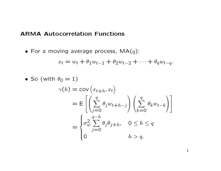
ARMA Autocorrelation Functions
- For a moving average process, MA(q):
xt = wt + θ1wt−1 + θ2wt−2 + · · · + θqwt−q.
- So (with θ0 = 1)
γ(h) = cov
- xt+h, xt
- = E
q
- j=0
θjwt+h−j
q
- k=0
θkwt−k
=
σ2
w q−h
- j=0