Arithmetic Division Distributed Arithmetic Newton Raphson Newton - - PowerPoint PPT Presentation

arithmetic
SMART_READER_LITE
LIVE PREVIEW

Arithmetic Division Distributed Arithmetic Newton Raphson Newton - - PowerPoint PPT Presentation

Advanced Digital IC Design Advanced Digital IC Design Number Representation Addition Multiplication Arithmetic Division Distributed Arithmetic Newton Raphson Newton Raphson CORDIC Unsigned Number Representation Example: Unsigned Number


slide-1
SLIDE 1

1

Advanced Digital IC Design

Arithmetic

Number Representation Advanced Digital IC Design Addition Multiplication Division Distributed Arithmetic Newton Raphson Newton Raphson CORDIC Unsigned Number Representation

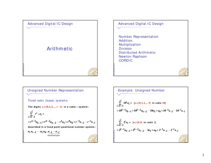
Fixed radix (base) systems

1 1 2 1 1 1 2 1 1 {0,1, 2, ... 1} l i i i k k k l k k l a r r

r a r a r a r a r a r a r a

×

− = − − − − − − − − ∈ − −

= = + + +

  • The digits

in a radix system :

1 1 0 1

.

i i l

a a a a a a

− − −

  • Fractional part

described in a fixed point positional num ber system :

Example: Unsigned Number

{ } {0,1, 2, ... 9} 10 1

10

a l i i i k

a

∈ −

=

in radix

{ } { 1 1 2 1 1 2 1 1 0,1} 2

10 10 10 10 10 2

i k k k l k k l l i i a

a a a a a a a

= − − − − − − − − − − ∈

= + + + =

  • in radix

1 1 2 1 1 2 1 1

2 2 2 2 2

i k k k l k i l

a a a a a a

= − − − − − − − − −

= + + +

slide-2
SLIDE 2

2

Signed Digit Number Representation

{ , 0, 1 } a r r l i α α ∈ − − − − … …

The digits in a radix system :

10

{ 4, 3, 0, 4, 5} 2 1

(3 1 5) 10 3 10 1 10 5 300 10 5 295

a i k i k

r a

× × ×

∈ − − =

− = − + = − + =

… …

Exam ple Radix 1 0 :

10 10

1 2

(3 1 5) 10 3 10 1 10 5 300 10 5 295 (3 . 1 5) 3 10 1 10 5 3 0.1 0.05 2.95

× ×

− −

+ + − = − + = − + =

Modified Booth’s recoding - a signed digit radix 4 representation

Two’s Complement

{0, 1 1}

2 2

l k i a − − ∈

The digits in a radix 2 system :

1 1 2 1 2 1 1 1 2 1 1

2 2 2 2 2 2 2 2

k i k i i k k k l k k l

a a a a a a a a

− = − − − − − − − − −

− × + × = = − + + +

  • described in a fixed point positional num ber system :

1 2 1 0 1

.

k k l

a a a a a a

− − − −

  • Fractional part

described in a fixed point positional num ber system :

  • Sign Bits

1 2 1 1 2 1 2

2 2 2 2 2 2 2

k k k k k k k

a a a a

=

− − − − − −

− + +

  • Sign Extension in Two’s Complement

1 2 1 1 1 2 1 1 2 1 1 1 1 2

2 2 2 2 2 2 2 2 2

k k k k k k k k k k k k k k

a a a a a a a a a a a

= +

− − − + − − − − − −

− + + + − + + +

  • Example:

10010 110010 1110010 11110010 00010 000010 0000010 00000010 = = = = = = = =

  • Addition is the most common arithmetic

ti i di it l

Addition

  • peration in digital processors

Also the basis of most other arithmetic

  • perations like

multiplication division division square root …

slide-3
SLIDE 3

3

Addition Ripple Carry Adder (RCA)

A0 B0 A2 A1 B2 B1 FA FA FA A3 B3 FA Ci,0 Co,0 Co,3 Co,2 Co,1 S0 S2 S1 S3

Critical Path through all adder cells Addition: Sign Extension

A0 B0 A2 A1 B2 B1 S S S FA FA FA S FA S FA S0 S2 S1 S3 S4

Adding More Numbers

Carry Ripple Adders in a Chain

A0 B0 A B

HA FA FA FA HA FA FA FA

D0 C0 D C

HA FA FA FA

S S0

Critical Path through 6 adder cells

Adding More Numbers

Carry Ripple Adders in a Tree

A0 B0 A B

HA FA FA FA HA FA FA FA

D C D0 C0

HA FA FA FA

S S0

Critical Path through 5 adder cells

slide-4
SLIDE 4

4

Adding More Numbers Carry Save Adder (CSA)

A0 B0 C0

FA FA FA FA HA FA FA FA

D0 Vect or

FA FA FA

S0 Vect or Merging Adder

Only One Critical Path (through 5 adder cells)

Pipelining

Ripple Carry Adders in a Chain

A0 B0 A B

HA FA FA FA HA FA FA FA

D0 C0 D C

R R R R R R R R R R

Critical Path through 4 adder cells

R = Register HA FA FA FA

S S0

Ripple Carry Adders in a Tree

Pipelining

A0 B0 A B

HA FA FA FA HA FA FA FA

D C D0 C0

R R R R R R R R R R

Lower Latency than the Chain Adder

R = Register HA FA FA FA

S S0

Latency

Latency: The number of clock cycles it takes before we se the result Latency time: Latency * cycle time

HA FA FA FA

A0 B0 A B D C D0 C0

HA FA FA FA

A0 B0 C0 A B C

R R R R R

HA FA FA FA HA FA FA FA

S S0

R R R R R R R R R R

HA FA FA FA HA FA FA FA

D0 D S S0

R R R R R

slide-5
SLIDE 5

5

Carry Save Adder (CSA) Pipelining

A0 B0 C0

FA FA FA FA HA FA FA FA

D0

R R R R R R R R R R R R R R R R

Register for both Sum and Carry needed Critical Path: 1 cell in CSA and 3 in vector merging

FA FA FA

S0 Vector Merging Adder

Carry Save Adder (CSA) with Carry Look Ahead (CLA)

Pipelining for fast addition

A0 B0C0

FA FA FA FA HA FA FA FA

D0 CLA

R R R R R R R R R R R R R R R R

Very Short Critical Path

R = Register CLA

S0 CLA Merging Adder

Vector Merging Adder - CLA

The CLA is done in blocks A common maximum is 4 bits per block Larger blocks are to complex

Co,2

CLA

A0 B0 A1 B1 A2 B2 Co,5

CLA

A3 B3 A4 B4 A5 B5 Co,8

CLA

A6 B6 A7 B7 A8 B8 C0 P0 S0 C1 P1 S1 C2 P2 S2 C3 P3 S3 C4 P4 S4 C5 P5 S5 C6 P6 S6 C7 P7 S7 C8 P8 S8

Generate & Propagate

A B C i S C o 0 Delete 0 Delete 1 1 0 Delete 1 1 0 Propagate 1 1 1 Propagate 1 1 0 Propagate 1 1 1 Propagate

FA

A B Ci Co

1 1 1 Propagate 1 1 1 Generate 1 1 1 1 1 Generate

S

slide-6
SLIDE 6

6 D A B P A B = ⊕ Delete, Propagate

Generate, Propagate

Functions

P A B G AB S A B C P C = ⊕ = = ⊕ ⊕ = ⊕ Propagate, Generate,

  • f A and B

1 1 1 1 1 1 1 A+ B B A

( ) ( )

  • C

AB AC BC AB A B C AB AB A B C G PC = + + = + + = = + + ⊕ = +

Redundant

Carry Look Ahead (CLA)

1 i,0 1 1 1

  • ,0

1

  • ,1

i,0

  • ,0

P P C P G G P C G C P C G C + + = + = + =

3 2 1 i,0 3 2 1 3 2 1 3 2 3

  • ,2

3

  • ,3

2 1 i,0 2 1 2 1 2 2

  • ,1

2

  • ,2

P P P P C P P P G P P G P G G P3 C G C P P P C P P G P G G P C G C + + + + = + = + + + = + =

Co,0 Co,3 Co,2 Co,1

2 1 i 0 2 1 2 1 2 2

  • 1

2

  • 2

1 i,0 1 1 1

  • ,0

1

  • ,1

i,0

  • ,0

P P P C P P G P G G P C G C P P C P G G P C G C P C G C + + + = + = + + = + = + =

Carry Look Ahead (CLA): Precharged

3 2 1 i,0 3 2 1 3 2 1 3 2 3

  • ,2

3

  • ,3

2 1 i,0 2 1 2 1 2 2

  • ,1

2

  • ,2

P P P P C P P P G P P G P G G P3 C G C + + + + = + =

P0

φ

P3 P2 P1

φ

G0 Ci G1 G2 G3

φ

Carry Look Ahead (CLA)

φ

P0 P3 P2 P1 G0 Ci G1 G2 G3

Alternative structure

φ

P0

φ

P3 P2 P1 G0 Ci G1 G2 G3

structure

slide-7
SLIDE 7

7

,3 3 ,2 3 2 3 1 2 3 1 2 3 ,0 1 2 3

3

  • i

C G C P G G P G P P G PP P C P PP P = + = + + + +

Carry Look Ahead (CLA): Manchester

VDD Co,3 Ci,0 G0 G1 G2 G3 P0 P1 P2 P3 ,0 ,0

  • i

C G PC = +

Logarithmic Adder

Look Ahead

  • ne step

Look Ahead two steps

  • 1:0

1:0 1:0 1:0

,1 1 1 ,0 1 1 1 ,0 1:0 1:0 ,0 ( ) ( ) ,2 2 2 ,1 2 2 1 1 2 1 ,0 2 2 1:0 2 1:0 ,0

( )

  • i

i Propagate P Generate G

  • i

i P G

C G PC G G P PP C G P C C G P C G P G G P P PP C G P G P P C = + = + + = + = + = + + + = + +

  • 2:1

,3 2 3 ,2 3 3 2 1 2

(

  • G

C G PC G P G G P = + = + +

  • 2:1

3 2 1 ,1 3 3 2:1 3 2:1 ,0

)

i

  • P

P P P C G PG P P C + = + +

  • Logarithmic Adder, 4 bit

P&G

Creation

A0 B G0 P0

1:0 1 1 1:0 1

G G G P P PP = + =

,0 i

G PC +

  • i

C G PC = +

Creation

B0

P&G

Creation

A2 B2

P&G

Creation

A1 B1 G1 P1 G2 P2

,1 1:0 1:0 ,0

  • i

C G P C = +

,2 2 2 1:0 2 1:0 ,0

  • i

C G PG P P C = + +

,0 ,0

  • i

P&G

Creation

A3 B3 G3 P3

= Gi:j Pi:j creation

,3 3 3 2:1 3 2:1 ,0

  • C

G PG P P C = + +

2:1 2 1 2 2:1 2 1

G G G P P P P = + =

Logarithmic Adder, 16 bit

P&G

Creation

A0 B0

P&G

Creation

A3 B

P&G

Creation

A2 B2

P&G

Creation

A1 B1 Co 3 Co,2 Co,1 Co,0

One step Look Ahead Two step Look Ahead

Creation

B3

P&G

Creation

A4 B4

P&G

Creation

A7 B7

P&G

Creation

A6 B6

P&G

Creation

A5 B5

P&G

Creation

A8 B8

P&G

Creation

A9 B9

  • ,3

Co,7 Co,6 Co,5 Co4 Co,9 Co,8

Four step Look Ahead

An N bit adder is computed in log (N) stages

P&G

Creation

A12 B12

P&G

Creation

A15 B15

P&G

Creation

A14 B14

P&G

Creation

A13 B13

P&G

Creation

A11 B11

P&G

Creation

A10 B10 Co,15 Co,14 Co,13 Co,12 Co,11 Co,10

Eight step Look Ahead

log2(N) stages Kogge-Stone adder

slide-8
SLIDE 8

8

Logarithmic Adder, 16 bit

P&G

Creation

A0 B0

P&G

Creation

A3 B

P&G

Creation

A2 B2

P&G

Creation

A1 B1 Co 3 Co,2 Co,1 Co,0

One step Look Ahead Two step Look Ahead

Creation

B3

P&G

Creation

A4 B4

P&G

Creation

A7 B7

P&G

Creation

A6 B6

P&G

Creation

A5 B5

P&G

Creation

A8 B8

P&G

Creation

A9 B9

  • ,3

Co,7 Co,6 Co,5 Co4 Co,9 Co,8

Four step Look Ahead

An N bit adder is computed in log (N) stages

P&G

Creation

A12 B12

P&G

Creation

A15 B15

P&G

Creation

A14 B14

P&G

Creation

A13 B13

P&G

Creation

A11 B11

P&G

Creation

A10 B10 Co,15 Co,14 Co,13 Co,12 Co,11 Co,10

Eight step Look Ahead

log2(N) stages Kogge-Stone adder

Other logarithmic adders

Kogge-Stone 17 cells Brent-Kung 12 cells 17 cells Fan out 2 12 cells Large fan out Sklansky adder Large fanout

Other logarithmic adders Carry Bypass

A B C i S C o 0 Delete 1 1 0 Delete 1 1 0 Propagate 1 1 1 Propagate 1 1 0 P t

A B

1 1 0 Propagate 1 1 1 Propagate 1 1 1 Generate 1 1 1 1 1 Generate

S Ci Co FA

  • i

A B C C ≠ = give Bypass carry if P=1 P A B = ⊕ Propagate,

  • i

A B C C = give independent of

slide-9
SLIDE 9

9

Carry Bypass

A0 B0 A1 B1 P0 P1

,1 ,0 1 1

  • i

C C A B A B = ≠ ≠ if and

FA FA Ci,0 Co,0 Co,1

,1 ,0 1 ,1 ,0

  • i
  • i

C C P P C C = that is if

  • therwise

independent of Bypass carry when P0 P1

Carry Bypass Adder

G1 G3 G0 G2 P1 P3 P0 P2 P1 P3 P0 P2 C0 C2 S1 S3 S0 S2

1 3 2 1 3 2

FA FA FA FA

C1 C3 Co3

P1 P3 P0 P2 Bypass if = 1

Otherwise Co3 independent of Co

Carry Bypass Adder

If A = B in at least one adder cell ⇒ Co not dependent on Ci

Setup S9 S11 S8 S10

FA FA FA FA

Setup S13 S15 S12 S14

FA FA FA FA

S5 S7 S4 S6

FA FA FA FA

Setup S1 S3 S0 S2

FA FA FA FA

Setup

If A ≠ B in all adders ⇒ Bypass Carry

Carry Select

Setup

FA FA FA FA FA FA FA FA

C C

"0" "1"

Sum Gen. S1 S3 S0 S2 Co,k+3 Ci,k

slide-10
SLIDE 10

10

Carry Select: Critical Path

Setup Setup Setup Setup

FA FA FA FA FA FA FA FA

Co,3 Ci,0 1

FA FA FA FA FA FA FA FA

Co,7 1

FA FA FA FA FA FA FA FA

Co,11 1

FA FA FA FA FA FA FA FA

1

Large area (two adders not needed in first stage)

Sum Gen. Sum Gen. Sum Gen. Sum Gen. S9 S11 S8 S10 S13 S15 S12 S14 S5 S7 S4 S6 S1 S3 S0 S2

Linear Carry Select

FA FA FA FA

Setup

FA FA FA FA

Setup

FA FA FA FA

Setup

FA FA FA FA

Setup

FA FA FA FA FA FA FA FA

Co,3 Ci,0 1

FA FA FA FA FA FA FA FA

Co,7 1

FA FA FA FA FA FA FA FA

Co,11 1

FA FA FA FA FA FA FA FA

1

The same number of bits in each stage

Sum Gen. Sum Gen. Sum Gen. Sum Gen. S9 S11 S8 S10 S13 S15 S12 S14 S5 S7 S4 S6 S1 S3 S0 S2

Square Root Carry Select

Setup Setup

Setup

Setup

FA FA FA

Co,1 Ci,0 1

FA FA FA FA FA FA

Co,4 1

FA FA FA FA FA FA FA FA

Co,8 1

FA FA FA FA FA FA FA FA

1

FA FA FA

Sum Sum Sum Gen. Sum Gen. S9 S11 S8 S10 S13 S12 S5 S7 S4 S6 S1 S3 S0 S2

Multiplication

The steps involved in multiplication

Partial product generation Accumulate the partial products

The maximum speed is O(log2W)

slide-11
SLIDE 11

11

Multipliers Iterative multipliers

One or a few partial products are processed each clock cycle Small area Slow

Hardware mapped multipliers

A complete multiplication each clock cycle Large area Fast

Iterative Multiplication

A simple multiplier Applicable to both Carry Ripple and Carry Save pp y pp y 3

2i

i i

P A B A b

=

= × = × × =

Unsigned Multiplication

a3 a2 a1 a0 b3 b2 b1 b0 a3 b0 a2 b0 a1 b0 a0 b0 a b a b a b a b

3 2 1 3 2 1

2 2 2 2 A b A b A b A b = × + × + × + ×

a3 b1 a2 b1 a1 b1 a0 b1 a3 b2 a2 b2 a1 b2 a0 b2 a3 b3 a2 b3 a1 b3 a0 b3 p6 p5 p4 p3 p2 p1 p0

Shifted partial products

Unsigned Multiplication

3 2 1 3 2 1

2 2 2 2 A b A b A b A b = × + × + × + ×

a3 a2 a1 a0 b3 b2 b1 b0 a3 b0 a2 b0 a1 b0 a0 b0 a3 b1 a2 b1 a1 b1 a0 b1 pp3

1

pp2

1

pp1

1

pp0

1

a3 b2 a2 b2 a1 b2 a0 b2

Rows in Multiplier

a3 b2 a2 b2 a1 b2 a0 b2 pp3

2

pp2

2

pp1

2

Pp0

2

a3 b3 a2 b3 a1 b3 a0 b3 p6 p5 p4 p3 P2 p1 p0

Multiplier

slide-12
SLIDE 12

12

Array Multiplier

xi xi yj yj

Basic cells

FA HA

Co Ci S S Co x3 x1 x0 x2 yj

HA FA FA HA

Partial Product Array Multiplier

b1 b0 a3 a1 a0 a2 a3 a1 a0 a2

Bit M lti li ti HA FA FA HA FA FA FA HA

b2 b3 a3 a1 a0 a2 a3 a1 a0 a2

aj ppj-1

i-1

bi

Bit Multiplication FA FA FA HA

b3 p3 p1 p0 p2 p5 p4 p6

FA

cout cin ppj

i

Array Multiplier: Critical Paths

HA FA FA HA FA FA FA HA FA FA FA HA

Carry Save Multiplier

Only one y critical path One extra adder S it bl f

FA FA FA HA FA FA FA HA HA HA HA HA

Suitable for CLA

FA FA FA HA FA FA HA HA

slide-13
SLIDE 13

13

Pipelining

y1 y0 x3 x1 x0 x2 x3 x1 x0 x2

HA FA FA HA FA FA FA HA

y2 x3 x1 x0 x2 x x x x

FA FA FA HA

y3 x3 x1 x0 x2 z3 z1 z0 z2 z5 z4 z6

HA HA HA HA

Pipelining

FA FA FA HA FA FA FA HA HA FA FA HA

Multiplier Floorplan

HA HA HA HA FA FA FA HA FA FA FA HA FA FA FA HA FA FA HA HA A B × =

Two’s Complement (Horner’s Rule)

Solved by sign extension

3 2 1 3 2 1 1 3 2 1 1 3 2 1 2 3 2 1 2 3 2 1

2 ( 2 2 2 ) 2 ( 2 2 2 ) 2 ( 2 2 2 ) b a a a a b a a a a b a a a a × − + + + + × − + + + + × − + + + + Need to be rewritten

2 3 2 1 3 3 2 1 3 3 2 1

2 ( 2 2 2 ) 2 ( 2 2 2 ) b a a a a b a a a a × + + + + − × − + + +

slide-14
SLIDE 14

14

3 3 2 1 3 3 2 1 3 3 2 1

2 ( 2 2 2 ) b a a a a − × − + + + =

Two’s Complement (Horner’s Rule)

LSB

3 3 2 1 3 3 2 1 3 3 2 1 3 3 2 1 3 3 2 1 3 3 3 2 1 3

2 (2 2 2 ) 2 ( 2 2 2 1) 2 ( 2 2 2 ) 2 b a a a a b a a a a b a a a a b = × − − − = = × − + + + + = = × − + + + + LSB Complemented

Multiplication (Horner’s Rule)

a3 a2 a1 a0 b3 b2 b1 b0

  • a3 b0

a2 b0 a1 b0 a0 b0 a b a b a b a b

[ ] 2 A b

  • a3 b1

a2 b1 a1 b1 a0 b1

  • a3 b2

a2 b2 a1 b2 a0 b2

  • a3 b3

a2 b3 a1 b3 a0 b3 b3 p6 p5 p4 p3 p2 p1 p0

1 1

[ ] 2 [ ] 2 A b A b × × × ×

3 3 2 1 3 3 3 2 1 3

2 ( 2 2 2 ) 2 b a a a a b × − + + + +

Multiplication (Horner’s Rule)

Negative MSBs solved with sign extension,

  • ne in each partial product

N t d if Not used if the result is truncated

Multiplication (Horner’s Rule)

Sign extension, one in each partial product

Note: Carry Ripple

Complement

3 0 3 1

a b a b +

“LSB one”

1 3 3 2

pp a b +

slide-15
SLIDE 15

15

Multiplication (Horner’s Rule)

Using Carry Save and Vector and Vector Merging Adder

CSA Cell

FA

A B C

(3, 2)

From stage

Often called:

S C To stage i+1 From stage i-1

Counts the # of

  • nes at the input

and compress it to a binary number Other are e.g.

Often called: 3-2 compressor (3, 2) counter

Other are e.g. (2, 2), (7, 3) … Used to form CSA trees

Wallace tree

Bit # First Stage Second Stage

Four 4-bit words to add HAs

(2, 2) Counters

FAs

Bit # 6 2 1 3 5 4 First Stage 6 2 1 3 5 4 First Stage Result Second Stage Result Second Stage 6 2 1 3 5 4 First Stage Result 6 2 1 3 5 4 Second Stage Result 6 2 1 3 5 4

Sum Carry

Wallace tree

HA HA 6 2 1 3 5 4

6 2 1 3 5 4

FA HA HA HA FA FA

CLA

Six adders (12 in CSA) Very high speed!

CLA

6 2 1 3 5 4

slide-16
SLIDE 16

16

Pipelined Wallace tree

6 2 1 3 5 4

6 2 1 3 5 4

FA HA HA HA FA FA

CLA

R R R R R R R R R R R R R

CLA

6 2 1 3 5 4

Very often combined with Booths modified encoding

64 Bit Wallace Tree Multiplier Booth´ s Modified Algorithm

0 1 2, 1,0 1,2

i i

x { , } y { , } ∈ ∈ − − Recode binary num bers to

Five possible digits in yi – radix 5 ? Overlapping radix 4 method Five digits require coding by 3 binary bits

Booth´ s Modified Algorithm

1 1 2

2 2 0 1 Example 6

k i k i i i k

X x x x { , } k

− − = −

= − × + × ∈ =

5 4 3 2 1 5 4 3 3 2 1 1 1 1 1

Example 6 32 16 8 4 2 16 2 4 2 2 2

i i i i

  • k

X x x x x x x X ( x x x ) ( x x x ) ( x x ) If y x x x x

+

= = − + + + + + = − + + + − + + + − + + = − + +

1 1 4 2 2 2 2

2 16 4 2 1 0 1 2 2 n, i even 4

i i i i- i i i i i k i k i

If y x x x X Y y y y y {- ,- , , , } Y y Y y

+ × = − =

+ + = = + + ∈ = × ⇒ =

1

i.e. Radix 4)

slide-17
SLIDE 17

17

Booth´ s Modified Algorithm

Examples:

i i 1 i i-1

y 2x x x

+

= − + +

Examples:

xi+1 xi xi-1 yi 1 1 1 1 1 1 2

X 01 11 01 10 (0) Y 02 01 02 02 X 00 10 01 11 (0) Y 01 02 02 01 = ⇒ = = ⇒ =

1

  • 2

1 1

  • 1

1 1

  • 1

1 1 1

X 10 11 10 10 (0) Y 01 00 01 02 = ⇒ =

There will always be at least one “0” in each pair

Booth´ s Modified Algorithm

0 1 0 1 5 0 1 0 1 5 x 0 1 1 1 7 x 2 1 7 x 0 1 1 1 7 x 2

  • 1

7 0 1 0 1 1 x 5 1 1 1 1 1 0 1 1

  • 5

0 1 0 1 2 x 5 + 0 1 0 1 2 x 4 x 5 0 1 0 1 4 x 5 0 0 1 0 0 0 1 1 + 0 0 0 0 0 x 5 0 0 1 0 0 0 1 1

  • 1 ⇒ two´ s complement conversion

2 ⇒ shift one step (multiply by two)

  • 2 ⇒ two´ s complement conversion + shift

yj-1 Xi+2 Xi Xi+1

Booth Booth Booth Booth Booth

Booth´ s Modified Algorithm

Adder Adder Adder Adder

yj+1 yj

Booth Coder Booth Booth MUX Booth MUX Booth MUX Booth MUX Booth Booth Booth Booth

1 × 2 ×

Adder Adder Adder Adder

yj+3 yj+2

Booth Coder Booth MUX Booth MUX Booth MUX Booth MUX

Booth´ s Modified Algorithm

Booth Muxes Booth Coders (one cell) Adders

slide-18
SLIDE 18

18

A0 B0 A3 A2 A1 B3 B2 B1 Adder/ Subtractor CTRL FA FA FA FA

CTRL B XOR 0 0 0 0 1 1 1 0 1 1 1 0

Overflow

Correct sum 3-bit two´s complement sum

1 3 2 1 2 3

Overflow h

Increase the dynamic range L ( dd ll )

1 3 2

changes the sign

Larger area (more adder cells) Scale down Decreases the dynamic range Use saturation logic Often a good solution

Overflow

1 1 3 1 1 3 1 1 3 1 1 3

A0 A4 A2 A1 A3 B0 B4 B2 B1 B3 C0 C4 C2 C1 C3 FA FA FA FA FA FA FA FA FA FA

A0 A4 A2 A1 A3 B0 B4 B2 B1 B3 C0 C4 C2 C1 C3 HA FA FA FA FA

1 1 3 1 1

  • 2

1 1 3 1 1 6

Increase the dynamic range

FA FA FA FA FA D0 D4 D2 D1 D3 FA FA FA FA FA S0 S4 S2 S1 S3

HA FA FA FA FA D0 D4 D2 D1 D3 HA FA FA FA FA S0 S4 S2 S1 S3 HA HA S6 S5 HA

Overflow

1 1 3 1 1 3 1 1 2 1 1 2

Scale down & l ft

1 1 3 1 1

  • 2

1 1 2 1 4

f(n) x(n) y(n)

scale up after Better than

  • verflow

f(n) x(n) y(n)

1 β β

slide-19
SLIDE 19

19

Overflow - Saturation

3 bit t ´

Saturation

Correct sum 3-bit two s complement sum

1 3 2 1 2 3

Saturation

3-bit saturated sum

2 3

Overflow change the sign

Correct sum

1 3 2 1 2

Cout-msb

Ci

b

Cout-msb

0 = NOF

From Adder

Saturation Arithmetic Cin-msb

Cin-msb

1 = POF Signbit

Saturated Output

Overflow if Cout-msb differs from Cin-msb Example: recursive filter

Limit Cycles

Two’s

Zero Input

Two s Complement Arithmetic Saturated Arithmetic

Source: Lars Wanhammar, “DSP Integrated circuits”

Fixed Coefficient Multiplication

a3 a2 a1 a0 1 1 a a a a a3 a2 a1 a0 1 1 a3 a2 a1 a0 a a a a a3 a2 a1 a0 a3 a2 a1 a0 p6 p6 p6 p5 p4 p3 p2 p1 p0 a3 a2 a1 a0 p6 p6 p6 p5 p4 p3 p2 p1 p0

a0 a0 a2 a1 a2 a1

HA HA HA

a3 a3

HA

slide-20
SLIDE 20

20 Bit-Serial

Serial Addition

Digit-Serial

i

a

i

b

1 + i

a

1 + i

b

i

s

1 + i

s

2 + i

s

i

cout

1 + i

cout

i

a

i

b

i

s

i

cout

Δ

b) a)

Δ

2 + i

a

2 + i

b

2 + i

cout

Bit-serial Multiplication

Coefficient ROM

LSB first in Sign Extension

h0(k) pi ai h1(k) h2(k) h3(k)

i

LSB first out

Fixed Coefficient Multiplication

pi ai 1 1 pi pi ai 1 1

Saves more than 1/ 2 of

pi ai 1 1

than 1/ 2 of the adders at an average

Example: Coef. from a Hilbert Filter

Bit-Parallel

a6 a7 a8 a9 a4 a5 a0 a1 a2 a3

HA FA FA HA FA FA

s10 s11 s12 s13 s14 s5 s6 s7 s9 s8

Binary point

s0 s1 s2 s3 s4

FA FA FA FA FA FA FA FA FA FA FA FA

a6 a7 a8 a4 a5 a0 a1 a2 a3 s15

Bit-Serial

FA FA

C = 00001101

slide-21
SLIDE 21

21

Signed Digit

A redundant representation where x∈{ -1,0,1} Example: 0 0 0 1 = 0 0 1 -1 = 0 1 -1 -1 … … A sequence of ones: 0 1 1 1 1 0 = 1 0 0 0 -1 0 16 + 8 + 4 + 2 = 32 - 2

Canonical Signed Digit (CSD)

A sequence of ones can be replaced with:

1 A “-1” at the least significant position of the sequence

  • 1. A

1 at the least significant position of the sequence.

  • 2. A “1” at the position to the left of the most significant

position of the sequence.

  • 3. Zeros between the “1” and the “–1”

1 1 1 1 1 1 1 1 1 1 1 1 1 1 1 1 1

  • 1

1 1 1 1

  • 1
  • 1
  • 1
  • 1
  • 1

Saves more than 2/ 3 of the adder cells at an average

Canonical Signed Digit

1 1 1 0 1 0 1 1 1 1 1 0 1 1 0 -1 1 1 1 1 1 1

ai si di ai

1 1 1 1 0 -1 0 -1 0 0 0 -1 0 -1 0 -1

  • 1
  • 1
  • 1

i

bi ci+1

i

ci reset

a)

i

set

i

bi ci ci+1

b)

pi ai

Signed Digit Representation

Booth’s modified algorithm Booth s modified algorithm For variable coefficients Canonical Signed Digit For fixed coefficients Optimal

slide-22
SLIDE 22

22

Distributed Arithmetic

Often used in summation of inner products for example Discrete Cosine Transform (DCT)

2 2 2 2 1 3 3 1 2 2 2 2

(0) (0) (1) (1) (2) (2) c c c c X x c c c c X x X c c c c x ⎡ ⎤ ⎡ ⎤ ⎡ ⎤ ⎢ ⎥ ⎢ ⎥ ⎢ ⎥ − − = × ⎢ ⎥ ⎢ ⎥ ⎢ ⎥ − − ⎢ ⎥ ⎢ ⎥ ⎢ ⎥

for example Discrete Cosine Transform (DCT)

2 2 2 2 3 1 1 3

( ) ( ) (3) (3) X x c c c c ⎢ ⎥ ⎢ ⎥ ⎢ ⎥ − − ⎢ ⎥ ⎣ ⎦ ⎣ ⎦ ⎣ ⎦

Distributed Arithmetic

Sum of inner products

1 N −1 0 0 1 1 2 2 N i i i

Y c x c x c x c x

− =

= = + +

  • ci are M-bit coefficients and xi are W-bit

numbers:

1 , 1 , 1 1

2

W j i i W i W j j

x x x

− − − − − =

= − + ×

numbers:

Distributed Arithmetic

Bits in the word 1 1 1 , 1 , 1

( 2 )

  • i

x N N W j i i i i W i W j

Y c x c x x

− − − − − − −

= = − + × =

∑ ∑ ∑

1 1 1 1 , 1 , 1 1 1 1 1

2

i i j N N W j i i W i i W j i i j N W N j

c x c x

= = = − − − − − − − = = = − − −

⎡ ⎤ ⎢ ⎥ = − + × = ⎢ ⎥ ⎣ ⎦ ⎡ ⎤

∑ ∑ ∑

Interchanged summation order

, 1 , 1 1

2

j i i W i i W j i j i

c x c x

− − − − = = =

⎡ ⎤ = − + × = ⎢ ⎥ ⎢ ⎥ ⎣ ⎦

∑ ∑ ∑

Same bit weight

Example: Distributed Arithmetic

Traditional summation order

0 0 1 1 2 2

Y c x c x c x = + + =

  • 1
  • 2

0 0,2 0 0,1 0 0,0

  • 1
  • 2

1 1,2 1 1,1 1 1,0

  • 2

2

  • 2

2 c x c x c x c x c x c x + + + + + +

  • 1
  • 2

2 2,2 2 2,1 2 2,0

  • 2

2 c x c x c x + +

Note: ci are M-bit constants and xi,j are single bits

slide-23
SLIDE 23

23

Interchanged

0 0 1 1 2 2

Y c x c x c x = + + = Example: Distributed Arithmetic

Interchanged summation

  • rder

1 2 0 0,2 0 0,1 0 0,0

2 2 c x c x c x

− −

− + + +

Sign bits

1 2 1 1,2 1 1,1 1 1,0 1 2 2 2,2 2 2,1 2 2,0

2 2 2 2 c x c x c x c x c x c x

− − − −

− + + + − + +

Interchanged summation order ( i )

x0,j x1,j x2,j ROM 1

Example: Distributed Arithmetic

(rewritten)

0 0,2 1 1,2 2 2,2

( ) c x c x c x − + + +

1 c2 1 c1 1 1 c1+c2 1 c0 1 1 c0+c2 1 1 c0+c1

Sign bits

1 0 0,1 1 1,1 2 2,1 2 0 0,0 1 1,0 2 2,0

( ) 2 ( ) 2 c x c x c x c x c x c x

− −

+ + + × + + + + ×

1 1 c0+c1 1 1 1 c0+c1+c2

Shift Accumulator

x0,j x1,j x2,j ROM

Example: Distributed Arithmetic

1 c2 1 c1 1 1 c1+c2 1 c0 1 1 c0+c2 x0,j

2N Word ROM

x2,j x1,j

REG

1 1 c0+c1 1 1 1 c0+c1+c2

LSB first

x0,j x1,j x2,j ROM Coeff. 0.00 1 0.10 c2

Example: Distributed Arithmetic

0,

  • 0. 1

1

j

x = 0.00 0 01 c =

1 0.01 c1 1 1 0.11 c1+c2 1 0.00 c0 1 1 0.10 c0+c2 1 1 0.01 c0+c1

1, 2,

. .01 10

j j

x x = =

1 2

0.01 0.10 c c = =

5 6

1 1 2 4 rom ro S rom u m m = + + =

1 1 1 0.11 c0+c1+c2

0.00 010 2 4 0. 0.0 0.0100 001 = + + =

slide-24
SLIDE 24

24

Restoring Division

436

  • 480

Subtract

  • 44

Negative 480 Restore (Add) 436 436

  • 240

Shift&Sub

15 x 25

0110110100 436 01111 15

240 Shift&Sub 196 01 Positive 196

  • 120

Shift&Sub 76 011 Positive 76

  • 60

Shift&Sub 16 0111 Positive 16 16

  • 30

Shift&Sub

  • 14

01110 Negative 30 Restore (Add) 16 01110 16

  • 15

Shift&Sub 1 011101 Positive

Quotient: 011101= 29 Reminder: 000001

0110110100 01111 Subtract 1111010100 Negative 01111 Restore (Add) 0110110100 110110100 01111 Shift&Sub

Restoring Division

0110110100 436 01111 15

01111 Shift&Sub 011000100 01 Positive 11000100 01111 Shift&Sub 01001100 011 Positive 1001100 01111 Shift&Sub 0010000 0111 Positive 010000 010000 01111 Shift&Sub 110010 01110 Negative 01111 Restore (Add) 010000 01110 100000 01111 Shift&Sub 000001 011101 Positive

Quotient: 011101= 29 Reminder: 000001

Non-restoring Division

436

  • 480

Subtract

  • 44

Negative 480 R t (Add) Restoring:

  • 1. Add the denominator
  • 2. Subtract half of it

480 Restore (Add) 436 436 436 Shift

  • 240

Shift&Sub 196 Non-restoring:

  • 1. Add half of the

denominator 436

  • 480

Subtract

  • 44

Negative 240 Shift&Add 196

  • 44

Non-restoring Division

0110110100 01111 Subtract 1111010100 Negative 01111 R t (Add) Restoring:

  • 1. Add the denominator
  • 2. Subtract half of it

01111 Restore (Add) 0110110100 0110110100 110110100 01111 Shift&Sub 011000100 Non-restoring:

  • 1. Add half of the

denominator 0110110100 01111 Subtract 1111010100 Negative 01111 Shift&Add 011000100 111010100

slide-25
SLIDE 25

25

Array Divider Non-restoring

1 CTRL A0 B0 A3 A2 A1 B3 B2 B1 FA FA FA FA

Selects ADD/SUB after shift

XOR ADD

Division by Reciprocation

To compute

z q d =

compute 1/ d multiply

Particularly efficient when several divisions by d

d 1 q z d = × 1 a b a b d d c e c e d d d ⎡ ⎤ ⎢ ⎥ ⎡ ⎤ = ⎢ ⎥ ⎢ ⎥ ⎣ ⎦ ⎢ ⎥ ⎢ ⎥ ⎣ ⎦

Newton Raphson

Efficient 1/ d computing

2

1 1 ( ) ; ( ) f x d f x x ′ = − = −

2 2 2 2

1 ( ( )) ( ) ( ) ( 1) ( ) ( ) ( ) ( ) 1 ( ( )) ( ) x x d f x i x i x i x i x i x i x i dx i f x i x i − + = − = − = + − ′ −

2 2

( ) ( 1) 2 ( ) ( ) x i x i x i dx i + = −

Convergence Speed up in NR

Convergence is slow in the beginning the number of bits doubles each iteration Speedup is possible use lookup table to set start value

slide-26
SLIDE 26

26

The CORDIC Algorithm

Iterative algorithm for circular rotations

Example: Derive sine, cosine … p ,

No multiplications CORDIC

COordinate Rotation DIgital Computer

Presented by Jack E. Volder 1959

Real Rotation

1 1

cos sin cos ( tan ) cos sin

i i i i i i i i i i i i i i

x x y x y y y x α α α α α α

+ +

= − = = − = + =

1 1

, x y

Find the x, y coordinates for a given l

1

cos ( tan ) Example: cos ( tan ) cos

i i i i

y x x x y x k x α α α α α = + = − = = × = = × angle True rotation

α

1

cos ( tan ) cos tan tan k x y y x x k x α α α α α = × = + = = × = = ×

, 1,0 x y =

Unit Circle

The rotation angle is restricted to

1

cos sin cos ( tan )

i i i i i

x x y x y α α α α

+ =

− = = =

Real Rotation

i.e. a shift

tan 2 i

i

α

= ±

1

cos ( tan ) ( ) ( ) cos sin cos tan ( tan ) 2

i i i i i i i i i i i i i i i i i i i i i i

x y k x y k x y y y x d y x α α α α α α α

− +

= − = = − = = − × = = + = = + × = t ) n ( a

i i i i

k y x α = +

However, multiplication with a constant

CORDIC: Pseudo Rotation

1 1

tan tan Example:

i i i i i i i i

x x y y y x α α

+ +

= − = + 1 1

, x y

No

1 1

p tan 1 tan tan x x y y y x α α α = − = = + =

Pseudo rotation True rotation

α

1

However the length 1 1 cos

i i

R R R α

+

> = = Ri Ri+1

No multiplication

Unit Circle

, 1,0 x y =

2 2 2 1

cos 1 1 tan cos 1 tan

i i i i i i

R R α α α α

+

⎧ ⎫ ⎪ ⎪ = = + = ⎨ ⎬ ⎪ ⎪ ⎩ ⎭ = +

i

slide-27
SLIDE 27

27

CORDIC: Pseudo Rotation

R2 R3

3 3

, x y

2 2

, x y

The Angle α is known De i e sing

R1 R2

1 1

, x y

, x y Derive x, y using three iterations where

1 2

45.0 26 87 1 .6 14. 4 . α α α α → = − − − − − −

  • ,

x y R0

87 α =

  • α

1

α

2

α

CORDIC: Three Iterations

The vector length R is increasing each

R2 R3

3 3

, x y

2 2

, x y

2 2 1 2 2 2 1 1

1 1 tan 1 tan 45 2 1.41 5 1 tan 2 1 tan 26 6 1 58

  • R

R R R R α α = = + = + = = = + = + = =

g iteration

R1 R2

1 1

, x y

, x y

2 1 1 2 2 3 2 2

1 tan 2 1 tan 26.6 1.58 2 5 85 1 tan 1 tan 14.0 1.63 2 32

  • R

R R R α α = + = + = = = + = + = =

, x y R0

87 α =

  • α

1

α

2

α

CORDIC Derive x3,y3

1 2 1

1 1 tan 1; tan ; tan 2 4 tan tan

i i i i

x x y y y x α α α α α

+

= = = = − + R2 R3

3 3

, x y

2 2

, x y

1 1 1 2 1 1

tan 1 1 1 1 1 1 2 2

i i i i

y y x x x y y y x x x y α

+ =

+ = − × = ⎧ ⎪ ⎨ = + × = ⎪ ⎩ ⎧ = − × = ⎪ ⎪ ⎨ R1

2

1 1

, x y

, x y

2 1 1 3 2 2 3 2 2

1 3 2 2 1 1 4 8 1 13 4 8 y y x x x y y y x ⎨ ⎪ = + × = ⎪ ⎩ ⎧ = − × = ⎪ ⎪ ⎨ ⎪ = + × = ⎪ ⎩ , x y R0

87 α =

  • α

1

α

2

α

1

30

  • Pos. Rot.

30 45 15

  • Neg. Rot.

15 26.6 11.6

  • Pos. Rot.

11 6 14 2 4 N R t α α α α α α = ⇒ − = − = − ⇒ − − = − + = ⇒

  • CORDIC

The sign determine the rotation direction

3 3

, , x y x y R R ≈

1 2 1 2

11.6 14 2.4

  • Neg. Rot.

The lengths are constant (precalculated) 1 2 5 2

i

R R R R α α α α − − − = − = − ⇒ = = =

  • R1

R3

, x y

3 3

R R

1 1

, x y

3 3

, x y

3

2 85 32 R = R0 R2

30 α =

  • ,

x y

2 2

, x y

α

1

α

2

α

slide-28
SLIDE 28

28

CORDIC Derive x3,y3

1 1

1 tan 1; tan 2 tan tan

  • i

i i i

x x y y y x α α α α

+

= = = − +

Negative Rotation

1 1 1 2 1 1

tan 1 1 1 1 1 3 2 2

i i i i

y y x x x y y y x x x y α

+ =

+ = − × = ⎧ ⎪ ⎨ = + × = ⎪ ⎩ ⎧ = + × = ⎪ ⎪ ⎨ R1 R3

, x y

1 1

, x y

3 3

, x y

2 1 1 3 2 2 3 2 2

1 1 2 2 1 11 4 8 1 7 4 8 y y x x x y y y x ⎨ ⎪ = − × = ⎪ ⎩ ⎧ = − × = ⎪ ⎪ ⎨ ⎪ = + × = ⎪ ⎩ R0 R2

30 α =

  • ,

x y

2 2

, x y

α

1

α

2

α

1 32 ( ) ( 0) ( 0) x y = =

CORDIC

New start vector

(No need for multiplication)

1

1 ( tan )

i i i i i

x x y R α

+ =

Start at

3 3 3

( ) ( ,0) ( ,0 , ) 85 ( ) , , ( ) x y x R y x y = = ⇒ ≈

3 3

, x y 1 3 2 2

1 ( tan ) 32 1 32 11 ( ) 85 4 85 8

i i i i i

y y x R x x y α

+ =

+ ⎧ = × − × = × ⎪ ⎪ ⎨

, x y

3 3

, y

, x y

30 α =

  • 3

2 2

32 1 32 7 ( ) 85 4 85 8 y y x ⎨ ⎪ = × + × = × ⎪ ⎩

Sine and Cosine

1 1

1 1 ( tan ); ( tan )

i i i i i i i i i i

x x y y y x R R α α

+ +

= − = +

3

cos cos

i

x α α = ≈

∑ ∑

3 2 2 3 1 2 1 2 2 2

32 1 32 11 ( ) 0.844 85 4 85 8 32 1 32 cos( ) sin 7 ( ) 0.537 85 4 85 8 ( ) x x y y y x α α α α α α ⎧ = × − × = × = = ⎪ ⎪ ⎨ ⎪ = × + × = × = − + = − ⎩ + ⎪

3

s n i i s n

i

y α α = ≈

∑ 30 α =

  • sin

tan tan ; (division needed) cos

i i i

α α α α = ≈

∑ ∑

Basic CORDIC Rotations

How to choose the angles Shifts Angles Prestored Vector lengths Ri are also Prestored

1 2

tan 1 1 tan 2 1 tan α α α = = =

1 2

arctan 1 45 1 arctan 26.6 2 1 arctan 14 0

  • α

α α = = = = = =

2 3 4

tan 4 1 tan 8 1 tan 16 α α α = =

2 3 4

arctan 14.0 4 1 arctan 7.1 8 1 arctan 3.6 16

  • α

α α = = = = = =

slide-29
SLIDE 29

29

Basic CORDIC Rotations

1

1 2

i i i i i

x x d y

+ =

Each CORDIC iteration require 3 ADD/ SUB 2 Shifts

1 1

2 1 2 1 arctan 2

i i i i i i i i i

y y d x d α α

+ +

= + = − 2 sign( )

i i

d α =

CORDIC Hardware: Iterative

ADD SUB X REG

Each CORDIC iteration require 3 ADD/ SUB 2 Shifts

ADD SUB Y REG Shift Shift ADD SUB REG

α

Lookup table

CORDIC Hardware: Unrolled

ADD SUB ADD SUB ADD SUB

x0 y0

Sign bit

α

α −

3 1 2

cos( ) x α α α = + +

3 1 2

sin( ) y α α α = + +

ADD SUB ADD SUB ADD SUB ADD SUB ADD SUB ADD SUB

1/2

x1

1/2

y1

Sign bit

α α −

1

α −

ADD SUB ADD SUB ADD SUB

1/4

x2

1/4

y2 x3 y3

Sign bit 1 2

α α α α − − −

1

α α α − −

2

α −

CORDIC Summary

The CORDIC algorithm is used for Polar/ rectangular conversion Polar/ rectangular conversion sine, cosine, tangent … arcsine, arcos, arctangent … Hyperbolic functions Division Square-root Square root … No multiplications needed One bit accuracy per iteration

slide-30
SLIDE 30

30

Binary Shifter

Bit-Slice

A0 A3 A2 A1 A

Four bit shifter

Right Left NOP Right Left NOP Q3 Q2 Q2 Q0 Q

Binary Shifter

A0 A3 A2 A1 A0 A3 A2 A1 A3 A Right Left

3

A0 A0 A2 A1 A2 A1 A3

Logarithmic Shifter

A6 A7 A3 A4 A5 A2 A0 A1 S1 S1 S2 S2 S4 S4

Example S= 101 (Shift 6 bit left)

A

6

A

7

A

3

A

4

A

5

A

2

A A

1

S

1

S

1 0 1 w ill

  • pen

S

1

S

2

S

2

S

4

S

4

A

7

A

7

A

7

A

7

A

7

A

7

A

6

A

5