
SLIDE 1
Nonlinear System Identification: A Palette from Off-white to Pit-black
Lennart Ljung Automatic Control, ISY, Linköpings Universitet
Lennart Ljung Brussels Workshop, April 25, 2017 Nonlinear System Identification
AUTOMATIC CONTROL REGLERTEKNIK LINKÖPINGS UNIVERSITET
The Problem
2(47)
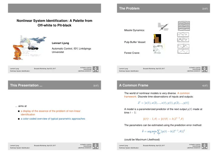
Missile Dynamics:
1 2 3 4 5 6 7 8 9 10 −5 5 Tunn: measurement; Tjock: simulation y1 1 2 3 4 5 6 7 8 9 10 −0.5 0.5 y2 1 2 3 4 5 6 7 8 9 10 −0.5 0.5 y3 1 2 3 4 5 6 7 8 9 10 −100 100 y4 1 2 3 4 5 6 7 8 9 10 −200 200 y5 [s]Pulp Buffer Vessel:
100 200 300 400 500 600 5 10 15 20 25 OUTPUT #1 100 200 300 400 500 600 10 15 20 INPUT #1Forest Crane:
100 200 300 400 500 600- 4
- 2
- 1
- 0.5
Lennart Ljung Brussels Workshop, April 25, 2017 Nonlinear System Identification
AUTOMATIC CONTROL REGLERTEKNIK LINKÖPINGS UNIVERSITET
This Presentation ...
3(47)
... aims at a display of the essence of the problem of non-linear identification a color-coded overview of typical parametric approaches
Lennart Ljung Brussels Workshop, April 25, 2017 Nonlinear System Identification
AUTOMATIC CONTROL REGLERTEKNIK LINKÖPINGS UNIVERSITET
A Common Frame
4(47)
The world of nonlinear models is very diverse. A common framework: Discrete time observations of inputs and outputs:
Zt = [u(1), u(2), ..., u(t), y(1), y(2), ..., y(t)]
A model is a parameterized predictor of the next output y(t) made at time t − 1:
ˆ y(t|t − 1, θ) = ˆ y(t|θ) = h(Zt−1, θ)
The parameters can be estimated using the prediction error method:
ˆ θ = arg min
θ ∑ t
y(t) − h(Zt−1, θ)2
(could be Maximum Likelihood)
Lennart Ljung Brussels Workshop, April 25, 2017 Nonlinear System Identification
AUTOMATIC CONTROL REGLERTEKNIK LINKÖPINGS UNIVERSITET