
SLIDE 1
1
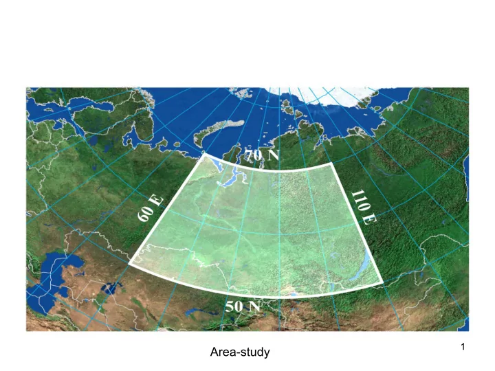
Area-study
Area-study DATA the daily observational data - - PowerPoint PPT Presentation
1 Area-study DATA the daily observational data (ftp://ftp.cdc.noaa.gov/pub/data/gsod/) at 169 stations during 19762006 the SCAND, NAO and ENSO teleconnection indices (http:// www.cpc.ncep.noaa.gov) describing the global circulation
1
Area-study
2
169 stations during 1976–2006
www.cpc.ncep.noaa.gov) describing the global circulation
Interregional territorial Administration of Federal Service for Hydrometeorology and Environmental Monitoring (West-Siberian AHEM)
(http://www.esrl.noaa.gov/psd/data/gridded/data.20thC_ReanV2.html)
1Ippolitov I.I., 2Gorbatenko V.P., 1Kabanov M.V., 1Loginov S.V., 1Podnebesnych N.V.
1Institute of Monitoring of Climatic and Ecological Systems, SB RAS, Tomsk, Russia 2High voltages research institute at Tomsk Polytechnic University, Tomsk, Russia
4
The spatial distribution of annual temperature trend Ttr (0C/decade) on Siberian region in 1976-2006
The distribution function of Ttr The probability density function of Ttr 169 Station
5
y = 0,023x - 2,8523
1976 1979 1982 1985 1988 1991 1994 1997 2000 2003 2006
Spatial averaged temperature T, oC
Year-to-year changes in the spatial averaged annual temperature T and its trend Ttr .Trend is significant in terms of 0.05 T=0.036 t – 2.49
6
Spatial averaged temperature and its linear trends for each month
7
The selected trajectories of cyclones (I÷VII) entrance to the region ‘Sib’ (white line)
8
30 35 40 45 50 55 60 65 70 75 1976 1978 1980 1982 1984 1986 1988 1990 1992 1994 1996 1998 2000 2002 2004 2006
The total number of cyclones nZ, which income to the region ‘Sib’ by synoptic maps. Trend is significant in terms of 0.05
Number of Cyclones nZ
nZ= -0.14 t – 2.85
9
y = -0,02+1000,8
996 997 998 999 1000 1001 1002 1003 1004 1976 1978 1980 1982 1984 1986 1988 1990 1992 1994 1996 1998 2000 2002 2004 2006 Year-to-year changes in the spatial averaged annual pressure centre of cyclones Pc and its trend Pctr Trend is not significant in terms of 0.05
Pressure Centre of Cyclones, hPa
Pc= -0.02 t + 1000
10
Variability in the number of cyclones for West (blue), North (red) and South (green) direction. The equations of regression are shown
y = -0,06x + 10,8 y = 0,14x + 17,6 y = -0,21x + 19,3
5 10 15 20 25 30 35 40 1976 1978 1980 1982 1984 1986 1988 1990 1992 1994 1996 1998 2000 2002 2004 2006
The Total Number of Cyclones Nz= 0,14 (±0,12) t + 17,6 Nz= -0,21 (±0,07) t + 19,3 Nz= -0,06 (±0,09) t + 10,8
11
wavelet spectra of the Variabilities of cyclones for South (a) and West (b) direction. a) b)
12
y = 0,04x + 998,9 y = 0,05x + 994,3 y = -0,09x + 1007,3
985,0 990,0 995,0 1000,0 1005,0 1010,0 1015,0 1976 1978 1980 1982 1984 1986 1988 1990 1992 1994 1996 1998 2000 2002 2004 2006
Variability in the pressure centre of cyclones for West (blue), North (red) and South (green) direction. The equations of regression are shown
Pressure Centre of Cyclones, hPa Pc= 0,05 (±0,07) t + 994,3 Pc= -0,09 (±0,05) t + 1007,3 Pc= 0,04 (±0,10) t + 998,9
13
Gulev S.K. et al Climate Dynamics, 2001, 17, 795-809
14
93) for north of 600N (dotted lines) and for 300–600N (dashed lines). To display both time series on the same scale, counts for the 300– 600N zonal band have been divided by two. Serreze M.C. et al J. Climate, 1997,v10, 453–464
15
January Jule The mean climatological locations of zones baroclinity between 1979-2008,
16 Matthias Zahn, and Hans von Storch, Geophysical Research Letters, 2008, v. 35, L22702 Polar low density distribution. Detected polar lows per 250 km2
17
(counts per 105 km2) Xiangdong Zhang, et al, Journal of Climate, Volume 17, Issue 12 (June 2004) 2300–2317
18
January Jule The mean climatological position of the Arctic and polar fronts between 1979-2008, obtained by calculating grad T at the grid 497gPa 1.125 ° x 1.125 °
700N for a) cyclone count (no. of events), b) MTG Paciorek C. J. et al J. Climate, 2002, v15, 7, 1573-1990 a) b)
20
Arctic front Polar front MTG (60,80) MTG (30,50) MTG indices are calculated by data from Reanalysis 20th Century
21
Table 2 Correlation between temperature and selected teleconnection indices
22
Table 3 Correlation between temperature and selected regional circulation values
23
24
Correlation between temperature and SCAND
25
Correlation between temperature and NAO
26
Correlation between temperature and SOI
27