Applications of Renormalization Group Methods in Nuclear Physics 3 - - PowerPoint PPT Presentation

Applications of Renormalization Group Methods in Nuclear Physics – 3

Dick Furnstahl

Department of Physics Ohio State University

HUGS 2014

Outline: Lecture 3

Lecture 3: Effective field theory

Recap from lecture 2: How SRG works Motivation for nuclear effective field theory Chiral effective field theory Universal potentials from RG evolution Extra: Quantitative measure of perturbativeness

Outline: Lecture 3

Lecture 3: Effective field theory

Recap from lecture 2: How SRG works Motivation for nuclear effective field theory Chiral effective field theory Universal potentials from RG evolution Extra: Quantitative measure of perturbativeness

Flow equations in action: NN only

In each partial wave with ǫk = 2k2/M and λ2 = 1/√s

dVλ dλ (k, k′) ∝ −(ǫk − ǫk′)2Vλ(k, k′) +

• q

(ǫk + ǫk′ − 2ǫq)Vλ(k, q)Vλ(q, k′)

Flow equations in action: NN only

In each partial wave with ǫk = 2k2/M and λ2 = 1/√s

dVλ dλ (k, k′) ∝ −(ǫk − ǫk′)2Vλ(k, k′) +

• q

(ǫk + ǫk′ − 2ǫq)Vλ(k, q)Vλ(q, k′)

Flow equations in action: NN only

In each partial wave with ǫk = 2k2/M and λ2 = 1/√s

dVλ dλ (k, k′) ∝ −(ǫk − ǫk′)2Vλ(k, k′) +

• q

(ǫk + ǫk′ − 2ǫq)Vλ(k, q)Vλ(q, k′)

Flow equations in action: NN only

In each partial wave with ǫk = 2k2/M and λ2 = 1/√s

dVλ dλ (k, k′) ∝ −(ǫk − ǫk′)2Vλ(k, k′) +

• q

(ǫk + ǫk′ − 2ǫq)Vλ(k, q)Vλ(q, k′)

Flow equations in action: NN only

In each partial wave with ǫk = 2k2/M and λ2 = 1/√s

dVλ dλ (k, k′) ∝ −(ǫk − ǫk′)2Vλ(k, k′) +

• q

(ǫk + ǫk′ − 2ǫq)Vλ(k, q)Vλ(q, k′)

Flow equations in action: NN only

In each partial wave with ǫk = 2k2/M and λ2 = 1/√s

dVλ dλ (k, k′) ∝ −(ǫk − ǫk′)2Vλ(k, k′) +

• q

(ǫk + ǫk′ − 2ǫq)Vλ(k, q)Vλ(q, k′)

Flow equations in action: NN only

In each partial wave with ǫk = 2k2/M and λ2 = 1/√s

dVλ dλ (k, k′) ∝ −(ǫk − ǫk′)2Vλ(k, k′) +

• q

(ǫk + ǫk′ − 2ǫq)Vλ(k, q)Vλ(q, k′)

Flow equations in action: NN only

In each partial wave with ǫk = 2k2/M and λ2 = 1/√s

dVλ dλ (k, k′) ∝ −(ǫk − ǫk′)2Vλ(k, k′) +

• q

(ǫk + ǫk′ − 2ǫq)Vλ(k, q)Vλ(q, k′)

Flow equations in action: NN only

In each partial wave with ǫk = 2k2/M and λ2 = 1/√s

dVλ dλ (k, k′) ∝ −(ǫk − ǫk′)2Vλ(k, k′) +

• q

(ǫk + ǫk′ − 2ǫq)Vλ(k, q)Vλ(q, k′)

Flow equations in action: NN only

In each partial wave with ǫk = 2k2/M and λ2 = 1/√s

dVλ dλ (k, k′) ∝ −(ǫk − ǫk′)2Vλ(k, k′) +

• q

(ǫk + ǫk′ − 2ǫq)Vλ(k, q)Vλ(q, k′)

Flow equations in action: NN only

In each partial wave with ǫk = 2k2/M and λ2 = 1/√s

dVλ dλ (k, k′) ∝ −(ǫk − ǫk′)2Vλ(k, k′) +

• q

(ǫk + ǫk′ − 2ǫq)Vλ(k, q)Vλ(q, k′)

Flow equations in action: NN only

In each partial wave with ǫk = 2k2/M and λ2 = 1/√s

dVλ dλ (k, k′) ∝ −(ǫk − ǫk′)2Vλ(k, k′) +

• q

(ǫk + ǫk′ − 2ǫq)Vλ(k, q)Vλ(q, k′)

Flow equations in action: NN only

In each partial wave with ǫk = 2k2/M and λ2 = 1/√s

dVλ dλ (k, k′) ∝ −(ǫk − ǫk′)2Vλ(k, k′) +

• q

(ǫk + ǫk′ − 2ǫq)Vλ(k, q)Vλ(q, k′)

Flow equations in action: NN only

In each partial wave with ǫk = 2k2/M and λ2 = 1/√s

dVλ dλ (k, k′) ∝ −(ǫk − ǫk′)2Vλ(k, k′) +

• q

(ǫk + ǫk′ − 2ǫq)Vλ(k, q)Vλ(q, k′)

Basics: SRG flow equations

[e.g., see arXiv:1203.1779]

Transform an initial hamiltonian, H = T + V, with Us:

Hs = UsHU†

s ≡ T + Vs ,

where s is the flow parameter. Differentiating wrt s:

dHs ds = [ηs, Hs] with ηs ≡ dUs ds U†

s = −η† s .

ηs is specified by the commutator with Hermitian Gs:

ηs = [Gs, Hs] ,

which yields the unitary flow equation (T held fixed),

dHs ds = dVs ds = [[Gs, Hs], Hs] . Very simple to implement as matrix equation (e.g., MATLAB)

Gs determines flow = ⇒ many choices (T, HD, HBD, . . . )

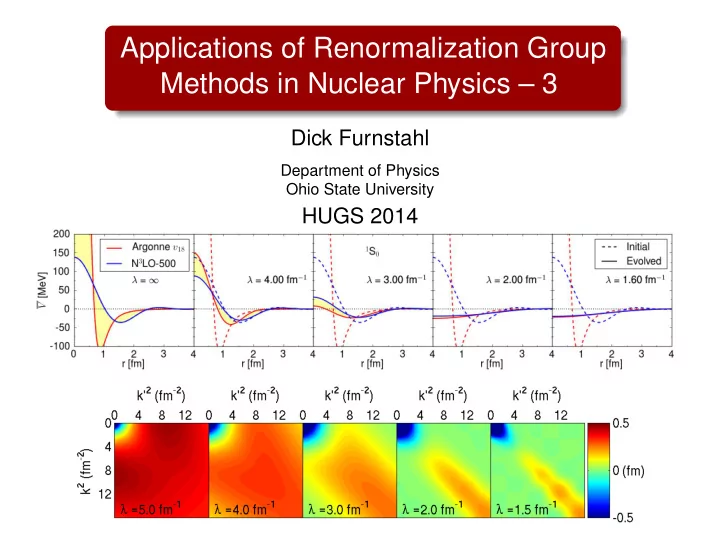
SRG flow of H = T + V in momentum basis

Takes H − → Hs = UsHU†

s in small steps labeled by s or λ

dHs ds = dVs ds = [[Trel, Vs], Hs] with Trel|k = ǫk|k and λ2 = 1/ √ s For NN, project on relative momentum states |k, but generic dVλ dλ (k, k′) ∝ −(ǫk − ǫk′)2Vλ(k, k′)+

• q

(ǫk + ǫk′ − 2ǫq)Vλ(k, q)Vλ(q, k′) Vλ=3.0(k, k′) 1st term 2nd term Vλ=2.5(k, k′) First term drives 1S0 Vλ toward diagonal: Vλ(k, k′) = Vλ=∞(k, k′) e−[(ǫk − ǫk′)/λ2]2 + · · ·

SRG flow of H = T + V in momentum basis

Takes H − → Hs = UsHU†

s in small steps labeled by s or λ

dHs ds = dVs ds = [[Trel, Vs], Hs] with Trel|k = ǫk|k and λ2 = 1/ √ s For NN, project on relative momentum states |k, but generic dVλ dλ (k, k′) ∝ −(ǫk − ǫk′)2Vλ(k, k′)+

• q

(ǫk + ǫk′ − 2ǫq)Vλ(k, q)Vλ(q, k′) Vλ=2.5(k, k′) 1st term 2nd term Vλ=2.0(k, k′) First term drives 1S0 Vλ toward diagonal: Vλ(k, k′) = Vλ=∞(k, k′) e−[(ǫk − ǫk′)/λ2]2 + · · ·

SRG flow of H = T + V in momentum basis

Takes H − → Hs = UsHU†

s in small steps labeled by s or λ

dHs ds = dVs ds = [[Trel, Vs], Hs] with Trel|k = ǫk|k and λ2 = 1/ √ s For NN, project on relative momentum states |k, but generic dVλ dλ (k, k′) ∝ −(ǫk − ǫk′)2Vλ(k, k′)+

• q

(ǫk + ǫk′ − 2ǫq)Vλ(k, q)Vλ(q, k′) Vλ=2.0(k, k′) 1st term 2nd term Vλ=1.5(k, k′) First term drives 1S0 Vλ toward diagonal: Vλ(k, k′) = Vλ=∞(k, k′) e−[(ǫk − ǫk′)/λ2]2 + · · ·

Outline: Lecture 3

Lecture 3: Effective field theory

Recap from lecture 2: How SRG works Motivation for nuclear effective field theory Chiral effective field theory Universal potentials from RG evolution Extra: Quantitative measure of perturbativeness

“Traditional” nucleon-nucleon interaction

(from T. Papenbrock)

Local nucleon-nucleon interaction for non-rel S-eqn

Depends on spins and isospins of nucleons; non-central

longest-range part is one-pion-exchange potential Vπ(r) ∝ (τ1·τ2)

• (3σ1 · ˆ

r σ2 · ˆ r − σ1 · σ2)(1 + 3 mπr + 3 (mπr)2 ) + σ1 · σ2 e−mπr r

Characterize operator structure of shorter-range potential

central, spin-spin, non-central tensor and spin-orbit {1, σ1 · σ2, S12, L · S, L2, L2σ1 · σ2, (L · S)2} ⊗ {1, τ1 · τ2}

Tensor = ⇒ deuteron wf is mixed S (L = 0) and D (L = 2) Non-zero quadrupole moment

• 300
• 200
• 100

100 200 1 2 3 4 5 6 S=0,T=1 S=1, T=0 deuteron

V(r) (MeV) r (fm)

The quantum numbers of the deuteron have the deepest potential well! proton-neutron L = 0 relative state Argonne v18

Problems with Phenomenological Potentials

The best potential models can describe with χ2/dof ≈ 1 all of the NN data (about 6000 points) below the pion production threshold. So what more do we need? Some drawbacks: Usually have very strong repulsive short-range part = ⇒ requires special (non-systematic) treatment in many-body calculations (e.g. nuclear structure). Difficult to estimate theoretical errors and range of applicability. Three-nucleon forces (3NF) are largely unconstrained and unsystematic models. How to define consistent 3NF’s and

• perators (e.g., meson exchange currents)?

Models are largely unconnected to QCD (e.g., chiral symmetry). Don’t connect NN and other strongly interacting processes (e.g., ππ and πN). Lattice QCD will be able to predict NN, 3N observables for high pion masses. How to extrapolate to physical pion masses? Alternative: Use Chiral Effective Field Theory (EFT)

QCD and Nuclear Forces

Quarks and gluons are the fundamental QCD dof’s, but . . . At low energies (low resolution), use “collective” degrees

• f freedom =

⇒ (colorless) hadrons. Which ones?

Different EFTs depending on scale of interest

Resolution

scale& separa)on&

DFT collective models CI ab initio LQCD constituent quarks

Effective theories

[H. Georgi, Ann. Rev. Nucl. Part. Sci. 43, 209 (1993)] One of the most astonishing things about the world in which we live is that there seems to be interesting physics at all scales. To do physics amid this remarkable richness, it is convenient to be able to isolate a set of phenomena from all the rest, so that we can describe it without having to understand everything. . . . We can divide up the parameter space of the world into different regions, in each of which there is a different appropriate description of the important physics. Such an appropriate description of the important physics is an “effective theory.” The common idea is that if there are parameters that are very large or very small compared to the physical quantities (with the same dimension) that we are interested in, we may get a simpler approximate description

• f the physics by setting the small parameters to zero and the large

parameters to infinity. Then the finite effects of the parameters can be included as small perturbations about this simple approximate starting point.

E.g., non-relativistic QM: c → ∞ E.g., chiral effective field theory (EFT): mπ → 0, MN → ∞ E.g., pionless effective field theory (EFT): mπ, MN → ∞ Goals: model independence (completeness) and error estimates

Classical analogy to EFT: Multipole expansion

If we have a localized charge distribution ρ(r) within a volume characterized by distance a, the electrostatic potential is φ(R) ∝

• d3r

ρ |R − r| If we expand 1/|R − r| for r ≪ R, we get the multipole expansion

• d3r

ρ |R − r| = q R + 1 R3

• i

RiPi + 1 6R5

• ij

(3RiRj − δijR2)Qij + · · · = ⇒ pointlike total charge q, dipole moment Pi, quadrupole Qij: q =

• d3r ρ(r)

Pi =

• d3r ρ(r) ri

Qij =

• d3r ρ(r)(3rirj − δijr 2)

Hierarchy of terms from separation of scales = ⇒ a/R expansion Can determine coefficients (LECs) by matching to actual distribution (if known) or comparing to experimental measurements Completeness = ⇒ model independent (cf. model of distribution)

Effective Field Theory Ingredients

General procedure for building an EFT . . .

1

Use the most general L with low-energy dof’s consistent with global and local symmetries of underlying theory

2

Declaration of regularization and renormalization scheme

3

Well-defined power counting = ⇒ small expansion parameter General procedures: QFT: trees + loops → renormalization Include long-range physics explicitly Short-distance physics captured in a few LEC’s (calculated from underlying

• r fit to data). Check naturalness.

Effective Field Theory Ingredients

General procedure for building an EFT . . .

1

Use the most general L with low-energy dof’s consistent with global and local symmetries of underlying theory What are the low-energy dof’s for QCD? What are the relevant symmetries?

2

Declaration of regularization and renormalization scheme What choices are there? Will we be able to use dimensional regularization?

3

Well-defined power counting = ⇒ small expansion parameter Usually Q/Λ. What are the QCD scales? General procedures: QFT: trees + loops → renormalization Include long-range physics explicitly Short-distance physics captured in a few LEC’s (calculated from underlying

• r fit to data). Check naturalness.

Outline: Lecture 3

Lecture 3: Effective field theory

Recap from lecture 2: How SRG works Motivation for nuclear effective field theory Chiral effective field theory Universal potentials from RG evolution Extra: Quantitative measure of perturbativeness

Symmetries of the QCD Lagrangian

Besides space-time symmetries and parity, what else? Is SU(3) color gauge “symmetry” in the EFT? Consider chiral symmetry . . .

LQCD = qLi/ DqL + qRi/ DqR − 1 2Tr GµνGµν−qRMqL − qLMqR / D ≡ / ∂ − igs/ GaT a ; T a = SU(3) Gell-Mann matrices M =

• mu

md

• SU(2) quark mass matrix

qL,R = 1 2(1 ± γ5)q , projection on left,right-handed quarks

mu and md are small compared to typical hadron masses

(5 and 9 MeV at 1 GeV renormalization scale vs. about 1 GeV) M ≈ 0 = ⇒ approximate SU(2)L ⊗ SU(2)R chiral symmetry

Chiral Symmetry of QCD

What happens if we have a symmetry of the Hamiltonian? Could have a multiplet of equal mass particles Could be a spontaneously broken (hidden) symmetry Experimentally we notice Isospin multiplets like p,n or Σ+,Σ−,Σ0 (that is, they have close to the same mass). So isospin symmetry is manifest. But we don’t find opposite parity partners for these states with close to the same mass. The “axial” part of chiral symmetry is spontaneously broken down! Isospin symmetry is “vectorial subgroup” with L = R The pions are pseudo-Goldstone bosons. The symmetry is explicitly broken by the quark masses, which means the pion is light (m2

π ≪ M2 QCD) but not massless.

Chiral symmetry relates states with different numbers of pions and dictates that pion interactions get weak at low energy = ⇒ pion as calculable long-distance dof in χEFT!

Effective Field Theory Ingredients

Specific answers for chiral EFT:

1

Use the most general L with low-energy dof’s consistent with the global and local symmetries of the underlying theory

2

Declaration of regularization and renormalization scheme

3

Well-defined power counting = ⇒ expansion parameters

Effective Field Theory Ingredients: Chiral NN

Specific answers for chiral EFT:

1

Use the most general L with low-energy dof’s consistent with the global and local symmetries of the underlying theory Left = Lππ + LπN + LNN chiral symmetry = ⇒ systematic long-distance pion physics

2

Declaration of regularization and renormalization scheme momentum cutoff and “Weinberg counting” (still unsettled!) = ⇒ define irreducible potential and sum with LS eqn use cutoff sensitivity as measure of uncertainties

3

Well-defined power counting = ⇒ expansion parameters use the separation of scales = ⇒ {p, mπ} Λχ with Λχ ∼ 1 GeV chiral symmetry = ⇒ VNN = ∞

ν=νmin cνQν with ν ≥ 0

naturalness: LEC’s are O(1) in appropriate units

Chiral Lagrangian

Unified description of ππ, πN, and NN · · · N Lowest orders [Can you identify the vertices?]: L(0) = 1 2∂µπ · ∂µπ − 1 2m2

ππ2 + N†

• i∂0 + gA

2fπ τσ · ∇π − 1 4f 2

π

τ · (π × ˙ π)

• N

− 1 2CS(N†N)(N†N) − 1 2CT(N†σN)(N†σN) + . . . , L(1) = N†

• 4c1m2

π − 2c1

f 2

π

m2

ππ2 + c2

f 2

π

˙ π2 + c3 f 2

π

(∂µπ · ∂µπ) − c4 2f 2

π

ǫijk ǫabc σiτa(∇j πb)(∇k πc)

• N

− D 4fπ (N†N)(N†στN) · ∇π − 1 2E (N†N)(N†τN) · (N†τN) + . . . Infinite # of unknown parameters (LEC’s), but leads to hierarchy

• f diagrams: ν = −4 + 2N + 2L +

i(di + ni/2 − 2) ≥ 0

LO: NLO:

renormalization of 1π-exchange renormalization of contact terms 7 LECs leading 2π-exchange 2 LECs

N2LO:

subleading 2π-exchange renormalization of 1π-exchange

N3LO:

sub-subleading 2π-exchange 3π-exchange (small) 15 LECs renormalization of contact terms renormalization of 1π-exchange

• V2N$=$V2N$$+V2N$+$V2N$+$V2N$+$…

Chiral expansion for the 2N force:

(0) (2) (3) (4)

Nucleon-nucleon force up to N3LO

Ordonez et al. ’94; Friar & Coon ’94; Kaiser et al. ’97; Epelbaum et al. ’98,‘03; Kaiser ’99-’01; Higa et al. ’03; …

Short4range'LECs'are' fi9ed'to'NN4data Single4nucleon'LECs'are' fi9ed'to'πN4data figure from H. Krebs

Chiral effective field theory for two nucleons

Epelbaum, Meißner, et al. Also Entem, Machleidt Organize by (Q/Λ)ν where Q = {p, mπ}, Λ ∼ 0.5–1 GeV LπN + match at low energy

Qν 1π 2π 4N

• ✂✁☎✄
• ✁

• 40

40 80 0.1 0.2 0.3 1S0 50 100 150 0.1 0.2 0.3 3S1 40 80 0.1 0.2 0.3 3P0 4 8 12 0.1 0.2 0.3 1D2

• 12
• 6

6 0.1 0.2 0.3 3D3

• 1.2
• 0.8
• 0.4

0.1 0.2 0.3 3G5

Chiral effective field theory for two nucleons

Epelbaum, Meißner, et al. Also Entem, Machleidt Organize by (Q/Λ)ν where Q = {p, mπ}, Λ ∼ 0.5–1 GeV LπN + match at low energy

Qν 1π 2π 4N Q0

• —

• ✁

• 40

40 80 0.1 0.2 0.3 1S0 50 100 150 0.1 0.2 0.3 3S1 40 80 0.1 0.2 0.3 3P0 4 8 12 0.1 0.2 0.3 1D2

• 12
• 6

6 0.1 0.2 0.3 3D3

• 1.2
• 0.8
• 0.4

0.1 0.2 0.3 3G5

Chiral effective field theory for two nucleons

Epelbaum, Meißner, et al. Also Entem, Machleidt Organize by (Q/Λ)ν where Q = {p, mπ}, Λ ∼ 0.5–1 GeV LπN + match at low energy

Qν 1π 2π 4N Q0

• —

Q1

• ✁

• 40

40 80 0.1 0.2 0.3 1S0 50 100 150 0.1 0.2 0.3 3S1 40 80 0.1 0.2 0.3 3P0 4 8 12 0.1 0.2 0.3 1D2

• 12
• 6

6 0.1 0.2 0.3 3D3

• 1.2
• 0.8
• 0.4

0.1 0.2 0.3 3G5

Chiral effective field theory for two nucleons

Epelbaum, Meißner, et al. Also Entem, Machleidt Organize by (Q/Λ)ν where Q = {p, mπ}, Λ ∼ 0.5–1 GeV LπN + match at low energy

Qν 1π 2π 4N Q0

• —

Q1 Q2

• ✁

• 40

40 80 0.1 0.2 0.3 1S0 50 100 150 0.1 0.2 0.3 3S1 40 80 0.1 0.2 0.3 3P0 4 8 12 0.1 0.2 0.3 1D2

• 12
• 6

6 0.1 0.2 0.3 3D3

• 1.2
• 0.8
• 0.4

0.1 0.2 0.3 3G5

Chiral effective field theory for two nucleons

Epelbaum, Meißner, et al. Also Entem, Machleidt Organize by (Q/Λ)ν where Q = {p, mπ}, Λ ∼ 0.5–1 GeV LπN + match at low energy

Qν 1π 2π 4N Q0

• —

Q1 Q2

• ✁

Q3

• 40

40 80 0.1 0.2 0.3 1S0 50 100 150 0.1 0.2 0.3 3S1 40 80 0.1 0.2 0.3 3P0 4 8 12 0.1 0.2 0.3 1D2

• 12
• 6

6 0.1 0.2 0.3 3D3

• 1.2
• 0.8
• 0.4

0.1 0.2 0.3 3G5

Chiral effective field theory for two nucleons

Epelbaum, Meißner, et al. Also Entem, Machleidt Organize by (Q/Λ)ν where Q = {p, mπ}, Λ ∼ 0.5–1 GeV LπN + match at low energy

Qν 1π 2π 4N Q0

• —

Q1 Q2

• ✁

Q3

Q4 many many

− → ∇

4

(15)

• 40

40 80 0.1 0.2 0.3 1S0 50 100 150 0.1 0.2 0.3 3S1 40 80 0.1 0.2 0.3 3P0 4 8 12 0.1 0.2 0.3 1D2

• 12
• 6

6 0.1 0.2 0.3 3D3

• 1.2
• 0.8
• 0.4

0.1 0.2 0.3 3G5

NN scattering up to N3LO (Epelbaum, nucl-th/0509032)

• 20

20 40 60

Phase Shift [deg]

1S0

50 100 150

3S1

• 30
• 20
• 10

1P1

• 20
• 10

10

Phase Shift [deg]

3P0

• 30
• 20
• 10

3P1

20 40

3P2

• 2

2 4

Phase Shift [deg]

ε1

5 10 15

1D2

• 30
• 20
• 10

3D1

50 100 150 200 250

• Lab. Energy [MeV]

10 20 30 40

Phase Shift [deg]

3D2

50 100 150 200 250

• Lab. Energy [MeV]
• 5

5

3D3

50 100 150 200 250

• Lab. Energy [MeV]
• 4
• 3
• 2
• 1

ε2

Theory error bands from varying cutoff over “natural” range

NN scattering up to N3LO (Epelbaum, nucl-th/0509032)

• 5
• 4
• 3
• 2
• 1

Phase Shift [deg]

1F3

0.5 1 1.5 2 2.5 3

3F2

• 3
• 2
• 1

3F3

0.5 1 1.5 2 2.5 3

Phase Shift [deg]

3F4

2 4 6

ε3

• 4
• 3
• 2
• 1

3G3

50 100 150 200 250

• Lab. Energy [MeV]
• 0.8
• 0.6
• 0.4
• 0.2

Phase Shift [deg]

3G5

50 100 150 200 250

• Lab. Energy [MeV]
• 1.5
• 1
• 0.5

1H5

50 100 150 200 250

• Lab. Energy [MeV]

0.1 0.2 0.3 0.4 0.5

3H4

Theory error bands from varying cutoff over “natural” range

Few-body chiral forces

At what orders? ν = −4 +

2N + 2L +

i(di + ni/2 − 2),

so adding a nucleon suppresses by Q2/Λ2. Power counting confirms 2NF ≫ 3NF > 4NF NLO diagrams cancel 3NF vertices may appear in NN and other processes Fits to the ci’s have sizable error bars

Status of chiral EFT forces [H. Krebs, TRIUMF Workshop (2014)]

• Zwei-Nukleon-Kraft

ührender Beitrag tur 1. Ordnung tur 2. Ordnung tur 3. Ordnung Drei-Nukleon-Kraft Vier-Nukleon-Kraft

Two-nucleon force Three-nucleon force Four-nucleon force

LO (Q0) NLO (Q2) N2LO (Q3) N3LO (Q4) accurate description of NN at least up to Elab ~ 200 MeV converged higher orders in progress not yet converged impact on few- & many-N systems? converged ??

Also in progress: versions with ∆ included = ⇒ better expansion?

Summary: Conceptual basis of (chiral) effective field theory

Separate the short-distance (UV) from long-distance (IR) physics = ⇒ defines a scale Exploit chiral symmetry = ⇒ hierarchical treatment of long-distance physics Use complete basis for short-distance physics = ⇒ hierarchy ` a la multipoles

Summary: Conceptual basis of (chiral) effective field theory

Separate the short-distance (UV) from long-distance (IR) physics = ⇒ defines a scale Exploit chiral symmetry = ⇒ hierarchical treatment of long-distance physics Use complete basis for short-distance physics = ⇒ hierarchy ` a la multipoles

QCD

T

ChPT

T

=

...

π

• −3

[H. Krebs]

Generate a nonrelativistic potential for many-body methods (controversies!)

• A

X

i=1

• ∇2

i

2mN + O(m−3

N )

• + V2N + V3N + V4N + . . .
• |Ψ = E|Ψ

derived&within&ChPT

m−3

Where/how do we draw the line? What if we draw it in different places?

How do we draw the line in an EFT? Regulators!

In coordinate space, define R0 to separate short and long distance In momentum space, use Λ to separate high and low momenta Much freedom how this is done = ⇒ different scales / schemes

How do we draw the line in an EFT? Regulators!

In coordinate space, define R0 to separate short and long distance In momentum space, use Λ to separate high and low momenta Much freedom how this is done = ⇒ different scales / schemes Non-local regulator in momentum (e.g., with n = 3 for N3LO): VCHPT(p, p′) − → e−(p2/Λ2)nVCHPT(p, p′)e−(p′2/Λ2)n Local regulator in coordinate space for long-range and delta function: Vlong(r) − → Vlong(r)(1 − e−(r/R0)4) and δ(r) − → Ce−(r/R0)4

Or local in momentum space [Gazit, Quaglioni, Navratil (2009)]

Rough relation: Λ = 450 . . . 600 MeV ⇐ ⇒ R0 = 1.0 . . . 1.2 fm

What does changing a cutoff do in an EFT?

(Local) field theory version in perturbation theory (diagrams) Loops (sums over intermediate states)

∆Λc

⇐ ⇒ LECs d dΛc

• Λc d3q

(2π)3 C0MC0 k2−q2+iǫ

+

C0(Λc)∝ Λc 2π2 +···

• = 0

Momentum-dependent vertices = ⇒ Taylor expansion in k2 Claim: Vlow k RG and SRG decoupling work analogously “Vlow k” SRG (“T” generator)

Outline: Lecture 3

Lecture 3: Effective field theory

Recap from lecture 2: How SRG works Motivation for nuclear effective field theory Chiral effective field theory Universal potentials from RG evolution Extra: Quantitative measure of perturbativeness

• S. Weinberg on the Renormalization Group (RG)

From “Why the RG is a good thing” [for Francis Low Festschrift] “The method in its most general form can I think be understood as a way to arrange in various theories that the degrees of freedom that you’re talking about are the relevant degrees of freedom for the problem at hand.” Improving perturbation theory; e.g., in QCD calculations Mismatch of energy scales can generate large logarithms RG: shift between couplings and loop integrals to reduce logs Nuclear: decouple high- and low-momentum modes Identifying universality in critical phenomena RG: filter out short-distance degrees of freedom Nuclear: evolve toward universal interactions Nuclear: simplifying calculations of structure/reactions Make nuclear physics look more like quantum chemistry! RG gains can violate conservation of difficulty! Use RG scale (resolution) dependence as a probe or tool

Flow of different N3LO chiral EFT potentials

1S0 from N3LO (500 MeV) of Entem/Machleidt 1S0 from N3LO (550/600 MeV) of Epelbaum et al.

Decoupling = ⇒ perturbation theory is more effective k|V|k+

• k′

k|V|k′k′|V|k (k2 − k′2)/m +· · · = ⇒ Vii+

• j

VijVji 1 (k2

i − k2 j )/m+· · ·

Flow of different N3LO chiral EFT potentials

3S1 from N3LO (500 MeV) of Entem/Machleidt 3S1 from N3LO (550/600 MeV) of Epelbaum et al.

Decoupling = ⇒ perturbation theory is more effective k|V|k+

• k′

k|V|k′k′|V|k (k2 − k′2)/m +· · · = ⇒ Vii+

• j

VijVji 1 (k2

i − k2 j )/m+· · ·

Approach to universality (fate of high-q physics)

Run NN to lower λ via SRG = ⇒ ≈Universal low-k VNN

Off-Diagonal Vλ(k, 0)

0.0 0.5 1.0 1.5 2.0 2.5 3.0 3.5

k [fm

−1]

−2.0 −1.5 −1.0 −0.5 0.0 0.5 1.0

Vλ(k,0) [fm]

550/600 [E/G/M] 600/700 [E/G/M] 500 [E/M] 600 [E/M]

λ = 5.0 fm

−1

1S0 q ≫ λ Vλ Vλ k < λ k′ < λ

= ⇒

C0

q ≫ λ (or λ) intermediate states = ⇒ replace with contact term: C0δ3(x − x′) [cf. Left = · · · + 1

2C0(ψ†ψ)2 + · · · ]

As resolution changes, shift high-k details to contacts, e.g., C0

Approach to universality (fate of high-q physics)

Run NN to lower λ via SRG = ⇒ ≈Universal low-k VNN

Off-Diagonal Vλ(k, 0)

0.0 0.5 1.0 1.5 2.0 2.5 3.0 3.5

k [fm

−1]

−2.0 −1.5 −1.0 −0.5 0.0 0.5 1.0

Vλ(k,0) [fm]

550/600 [E/G/M] 600/700 [E/G/M] 500 [E/M] 600 [E/M]

λ = 4.0 fm

−1

1S0 q ≫ λ Vλ Vλ k < λ k′ < λ

= ⇒

C0

q ≫ λ (or λ) intermediate states = ⇒ replace with contact term: C0δ3(x − x′) [cf. Left = · · · + 1

2C0(ψ†ψ)2 + · · · ]

As resolution changes, shift high-k details to contacts, e.g., C0

Approach to universality (fate of high-q physics)

Run NN to lower λ via SRG = ⇒ ≈Universal low-k VNN

Off-Diagonal Vλ(k, 0)

0.0 0.5 1.0 1.5 2.0 2.5 3.0 3.5

k [fm

−1]

−2.0 −1.5 −1.0 −0.5 0.0 0.5 1.0

Vλ(k,0) [fm]

550/600 [E/G/M] 600/700 [E/G/M] 500 [E/M] 600 [E/M]

λ = 3.0 fm

−1

1S0 q ≫ λ Vλ Vλ k < λ k′ < λ

= ⇒

C0

q ≫ λ (or λ) intermediate states = ⇒ replace with contact term: C0δ3(x − x′) [cf. Left = · · · + 1

2C0(ψ†ψ)2 + · · · ]

As resolution changes, shift high-k details to contacts, e.g., C0

Approach to universality (fate of high-q physics)

Run NN to lower λ via SRG = ⇒ ≈Universal low-k VNN

Off-Diagonal Vλ(k, 0)

0.0 0.5 1.0 1.5 2.0 2.5 3.0 3.5

k [fm

−1]

−2.0 −1.5 −1.0 −0.5 0.0 0.5 1.0

Vλ(k,0) [fm]

550/600 [E/G/M] 600/700 [E/G/M] 500 [E/M] 600 [E/M]

λ = 2.5 fm

−1

1S0 q ≫ λ Vλ Vλ k < λ k′ < λ

= ⇒

C0

q ≫ λ (or λ) intermediate states = ⇒ replace with contact term: C0δ3(x − x′) [cf. Left = · · · + 1

2C0(ψ†ψ)2 + · · · ]

As resolution changes, shift high-k details to contacts, e.g., C0

Approach to universality (fate of high-q physics)

Run NN to lower λ via SRG = ⇒ ≈Universal low-k VNN

Off-Diagonal Vλ(k, 0)

0.0 0.5 1.0 1.5 2.0 2.5 3.0 3.5

k [fm

−1]

−2.0 −1.5 −1.0 −0.5 0.0 0.5 1.0

Vλ(k,0) [fm]

550/600 [E/G/M] 600/700 [E/G/M] 500 [E/M] 600 [E/M]

λ = 2.0 fm

−1

1S0 q ≫ λ Vλ Vλ k < λ k′ < λ

= ⇒

C0

q ≫ λ (or λ) intermediate states = ⇒ replace with contact term: C0δ3(x − x′) [cf. Left = · · · + 1

2C0(ψ†ψ)2 + · · · ]

As resolution changes, shift high-k details to contacts, e.g., C0

Approach to universality (fate of high-q physics)

Run NN to lower λ via SRG = ⇒ ≈Universal low-k VNN

Off-Diagonal Vλ(k, 0)

0.0 0.5 1.0 1.5 2.0 2.5 3.0 3.5

k [fm

−1]

−2.0 −1.5 −1.0 −0.5 0.0 0.5 1.0

Vλ(k,0) [fm]

550/600 [E/G/M] 600/700 [E/G/M] 500 [E/M] 600 [E/M]

λ = 1.5 fm

−1

1S0 q ≫ λ Vλ Vλ k < λ k′ < λ

= ⇒

C0

q ≫ λ (or λ) intermediate states = ⇒ replace with contact term: C0δ3(x − x′) [cf. Left = · · · + 1

2C0(ψ†ψ)2 + · · · ]

As resolution changes, shift high-k details to contacts, e.g., C0

NN VSRG universality from phase equivalent potentials

Diagonal elements collapse where phase equivalent [Dainton et al, 2014]

1 2 3

k [fm−1 ]

15 15 30 45 60

δ(k) [degrees]

1 S0

(a)

1 2 3

k [fm−1 ]

40 40 80 120 160

δ(k) [degrees]

3 S1

(b)

1 2 3

k [fm−1 ]

10 20 30

δ(k) [degrees]

1 P1

(c)

1 2 3

k [fm−1 ]

1.2 0.9 0.6 0.3 0.0 0.3

V(k,k) [fm]

1 S0

(a) λ = ∞

1 2 3

k [fm−1 ]

2.5 2.0 1.5 1.0 0.5 0.0 0.5 1.0 1.5

V(k,k) [fm]

λ = ∞

3 S1

(b) 1 2 3

k [fm−1 ]

0.0 0.1 0.2 0.3 0.4 0.5 0.6

V(k,k) [fm]

λ = ∞

1 P1

(c)

NN VSRG universality from phase equivalent potentials

Diagonal elements collapse where phase equivalent [Dainton et al, 2014]

1 2 3

k [fm−1 ]

15 15 30 45 60

δ(k) [degrees]

1 S0

(a)

1 2 3

k [fm−1 ]

40 40 80 120 160

δ(k) [degrees]

3 S1

(b)

1 2 3

k [fm−1 ]

10 20 30

δ(k) [degrees]

1 P1

(c)

1 2 3

k [fm−1 ]

1.2 0.9 0.6 0.3 0.0 0.3

V(k,k) [fm]

1 S0

(a) λ = 1.5 fm−1

1 2 3

k [fm−1 ]

2.5 2.0 1.5 1.0 0.5 0.0 0.5 1.0 1.5

V(k,k) [fm]

3 S1

λ = 1.5 fm−1 (b) 1 2 3

k [fm−1 ]

0.0 0.1 0.2 0.3 0.4 0.5 0.6

V(k,k) [fm]

λ = 1.5 fm−1

1 P1

(c)

Use universality to probe decoupling

What if not phase equivalent everywhere? Use 1P1 as example (for a change :) Result: local decoupling!

1 2 3 4 5 6 7 8

klab [fm−1 ]

70 60 50 40 30 20 10

δ(klab) [degrees]

1 P1

(c) ISSP AV18

1 2 3 4 5 6 7 8

k [fm−1 ]

0.4 0.2 0.0 0.2 0.4 0.6

V(k,k) [fm]

1 P1

(c) ISSP λ =∞ AV18 λ =∞ ISSP λ = 1.5 AV18 λ = 1.5

1 2 3 4 5 6 7 8

klab [fm−1 ]

70 60 50 40 30 20 10

δ(klab) [degrees]

1 P1

(a) ISSP AV18

1 2 3 4 5 6 7 8

k [fm−1 ]

0.4 0.2 0.0 0.2 0.4 0.6

V(k,k) [fm]

1 P1

(b) ISSP λ =∞ AV18 λ =∞ ISSP λ = 1.5 fm−1 AV18 λ = 1.5 fm−1

Use universality to probe decoupling

What if not phase equivalent everywhere? Use 1P1 as example (for a change :) Result: local decoupling!

1 2 3 4 5 6 7 8

klab [fm−1 ]

70 60 50 40 30 20 10

δ(klab) [degrees]

1 P1

(c) ISSP AV18

1 2 3 4 5 6 7 8

k [fm−1 ]

0.4 0.2 0.0 0.2 0.4 0.6

V(k,k) [fm]

1 P1

(c) ISSP λ =∞ AV18 λ =∞ ISSP λ = 1.5 AV18 λ = 1.5

1 2 3 4 5 6 7 8

klab [fm−1 ]

90 80 70 60 50 40 30 20 10

δ(klab) [degrees]

1 P1

(a) ISSP AV18

1 2 3 4 5 6 7 8

k [fm−1 ]

0.4 0.2 0.0 0.2 0.4 0.6

V(k,k) [fm]

1 P1

(b) ISSP λ =∞ AV18 λ =∞ ISSP λ = 1.5 fm−1 AV18 λ = 1.5 fm−1

Outline: Lecture 3

Lecture 3: Effective field theory

Recap from lecture 2: How SRG works Motivation for nuclear effective field theory Chiral effective field theory Universal potentials from RG evolution Extra: Quantitative measure of perturbativeness

• S. Weinberg on the Renormalization Group (RG)

From “Why the RG is a good thing” [for Francis Low Festschrift] “The method in its most general form can I think be understood as a way to arrange in various theories that the degrees of freedom that you’re talking about are the relevant degrees of freedom for the problem at hand.” Improving perturbation theory; e.g., in QCD calculations Mismatch of energy scales can generate large logarithms RG: shift between couplings and loop integrals to reduce logs Nuclear: decouple high- and low-momentum modes Identifying universality in critical phenomena RG: filter out short-distance degrees of freedom Nuclear: evolve toward universal interactions Nuclear: simplifying calculations of structure/reactions Make nuclear physics look more like quantum chemistry! RG gains can violate conservation of difficulty! Use RG scale (resolution) dependence as a probe or tool

Flow of different N3LO chiral EFT potentials

1S0 from N3LO (500 MeV) of Entem/Machleidt 1S0 from N3LO (550/600 MeV) of Epelbaum et al.

Decoupling = ⇒ perturbation theory is more effective k|V|k+

• k′

k|V|k′k′|V|k (k2 − k′2)/m +· · · = ⇒ Vii+

• j

VijVji 1 (k2

i − k2 j )/m+· · ·

Flow of different N3LO chiral EFT potentials

3S1 from N3LO (500 MeV) of Entem/Machleidt 3S1 from N3LO (550/600 MeV) of Epelbaum et al.

Decoupling = ⇒ perturbation theory is more effective k|V|k+

• k′

k|V|k′k′|V|k (k2 − k′2)/m +· · · = ⇒ Vii+

• j

VijVji 1 (k2

i − k2 j )/m+· · ·

Convergence of the Born series for scattering

Consider whether the Born series converges for given z

T(z) = V + V 1 z − H0 V + V 1 z − H0 V 1 z − H0 V + · · ·

If bound state |b, series must diverge at z = Eb, where

(H0 + V)|b = Eb|b = ⇒ V|b = (Eb − H0)|b

Convergence of the Born series for scattering

Consider whether the Born series converges for given z

T(z) = V + V 1 z − H0 V + V 1 z − H0 V 1 z − H0 V + · · ·

If bound state |b, series must diverge at z = Eb, where

(H0 + V)|b = Eb|b = ⇒ V|b = (Eb − H0)|b

For fixed E, generalize to find eigenvalue ην [Weinberg]

1 Eb − H0 V|b = |b = ⇒ 1 E − H0 V|Γν = ην|Γν

From T applied to eigenstate, divergence for |ην(E)| ≥ 1:

T(E)|Γν = V|Γν(1 + ην + η2

ν + · · · )

= ⇒ T(E) diverges if bound state at E for V/ην with |ην| ≥ 1

Weinberg eigenvalues as function of cutoff Λ/λ

Consider ην(E = −2.22 MeV) Deuteron = ⇒ attractive eigenvalue ην = 1

Λ ↓ = ⇒ unchanged

2 3 4 5 6 7

Λ [fm

• 1]

0.5 1 1.5 2 2.5

| ην |

free space, η > 0

3S1 (Ecm = -2.223 MeV)

Weinberg eigenvalues as function of cutoff Λ/λ

Consider ην(E = −2.22 MeV) Deuteron = ⇒ attractive eigenvalue ην = 1

Λ ↓ = ⇒ unchanged

But ην can be negative, so V/ην = ⇒ flip potential

Weinberg eigenvalues as function of cutoff Λ/λ

Consider ην(E = −2.22 MeV) Deuteron = ⇒ attractive eigenvalue ην = 1

Λ ↓ = ⇒ unchanged

But ην can be negative, so V/ην = ⇒ flip potential

Weinberg eigenvalues as function of cutoff Λ/λ

Consider ην(E = −2.22 MeV) Deuteron = ⇒ attractive eigenvalue ην = 1

Λ ↓ = ⇒ unchanged

But ην can be negative, so V/ην = ⇒ flip potential Hard core = ⇒ repulsive eigenvalue ην

Λ ↓ = ⇒ reduced

2 3 4 5 6 7

Λ [fm

• 1]

0.5 1 1.5 2 2.5

| ην |

free space, η > 0 free space, η < 0

3S1 (Ecm = -2.223 MeV)

Weinberg eigenvalues as function of cutoff Λ/λ

Consider ην(E = −2.22 MeV) Deuteron = ⇒ attractive eigenvalue ην = 1

Λ ↓ = ⇒ unchanged

But ην can be negative, so V/ην = ⇒ flip potential Hard core = ⇒ repulsive eigenvalue ην

Λ ↓ = ⇒ reduced

In medium: both reduced

ην ≪ 1 for Λ ≈ 2 fm−1

= ⇒ perturbative (at least for particle-particle channel)

2 3 4 5 6 7

Λ [fm

• 1]

0.5 1 1.5 2 2.5

| ην |

free space, η > 0 free space, η < 0 kf = 1.35 fm

• 1, η > 0

kf = 1.35 fm

• 1, η < 0

3S1 (Ecm = -2.223 MeV)

Weinberg eigenvalue analysis of convergence

Born Series: T(E) = V + V 1 E − H0 V + V 1 E − H0 V 1 E − H0 V + · · ·

For fixed E, find (complex) eigenvalues ην(E) [Weinberg]

1 E − H0 V|Γν = ην|Γν = ⇒ T(E)|Γν = V|Γν(1+ην+η2

ν+· · · )

= ⇒ T diverges if any |ην(E)| ≥ 1

[nucl-th/0602060]

AV18 CD-Bonn N

3LO (500 MeV)

−3 −2 −1 1

Re η

−3 −2 −1 1

Im η 1S0

−3 −2 −1 1

Re η

−3 −2 −1 1

Im η AV18 CD-Bonn N

3LO

3S1− 3D1

Lowering the cutoff increases “perturbativeness”

Weinberg eigenvalue analysis (repulsive) [nucl-th/0602060]

−3 −2 −1 1

Re η

−3 −2 −1 1

Im η

Λ = 10 fm

• 1

Λ = 7 fm

• 1

Λ = 5 fm

• 1

Λ = 4 fm

• 1

Λ = 3 fm

• 1

Λ = 2 fm

• 1

N

3LO

1S0 1.5 2 2.5 3 3.5 4

Λ (fm

• 1)

−1 −0.8 −0.6 −0.4 −0.2

ην(E=0)

Argonne v18 N

2LO-550/600 [19]

N

3LO-550/600 [14]

N

3LO [13]

1S0

Lowering the cutoff increases “perturbativeness”

Weinberg eigenvalue analysis (repulsive) [nucl-th/0602060]

−3 −2 −1 1

Re η

−3 −2 −1 1

Im η

Λ = 10 fm

• 1

Λ = 7 fm

• 1

Λ = 5 fm

• 1

Λ = 4 fm

• 1

Λ = 3 fm

• 1

Λ = 2 fm

• 1

N

3LO

3S1− 3D1 1.5 2 2.5 3 3.5 4

Λ (fm

• 1)

−2 −1.5 −1 −0.5

ην(E=0)

Argonne v18 N

2LO-550/600

N

3LO-550/600

N

3LO [Entem]

3S1− 3D1

Lowering the cutoff increases “perturbativeness”

Weinberg eigenvalue analysis (ην at −2.22 MeV vs. density)

0.2 0.4 0.6 0.8 1 1.2 1.4

kF [fm

• 1]
• 1
• 0.5

0.5 1

ην(Bd)

Λ = 4.0 fm

• 1

Λ = 3.0 fm

• 1

Λ = 2.0 fm

• 1

3S1 with Pauli blocking

Pauli blocking in nuclear matter increases it even more!

at Fermi surface, pairing revealed by |ην| > 1