[PPT] - Applications of Renormalization Group Methods in Nuclear Physics 6 PowerPoint Presentation

SLIDE 1

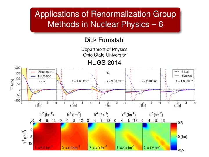
Applications of Renormalization Group Methods in Nuclear Physics – 6

Dick Furnstahl

Department of Physics Ohio State University

HUGS 2014

SLIDE 2

Outline: Lecture 6

Lecture 6: High-res. probes of low-res. nuclei

Recap: Running Hamiltonians Parton distributions as paradigm Summary and challenges Extra: High-res. probes of low-res. nuclei

SLIDE 3

Outline: Lecture 6

Lecture 6: High-res. probes of low-res. nuclei

Recap: Running Hamiltonians Parton distributions as paradigm Summary and challenges Extra: High-res. probes of low-res. nuclei

SLIDE 4

“Measuring” the QCD Hamiltonian: Running αs(Q2)

QCD α (Μ ) = 0.1184 ± 0.0007

s

Z

0.1 0.2 0.3 0.4 0.5

αs (Q)

1 10 100

Q [GeV]

Heavy Quarkonia e+e– Annihilation Deep Inelastic Scattering

July 2009

The QCD coupling is scale dependent (“running”): αs(Q2) ≈ [β0 ln(Q2/Λ2

QCD)]−1

The QCD coupling strength αs is scheme dependent (e.g., “V” scheme used on lattice, or MS) Extractions from experiment can be compared (here at MZ ):

0.11 0.12 0.13

α (Μ )

s

Z Quarkonia (lattice) DIS F2 (N3LO) τ-decays (N3LO) DIS jets (NLO) e+e– jets & shps (NNLO) electroweak fits (N3LO) e+e– jets & shapes (NNLO) Υ decays (NLO)

cf. QED, where αem(Q2) is

effectively constant for soft Q2: αem(Q2 = 0) ≈ 1/137 ∴ fixed H for quantum chemistry

SLIDE 5

Running QCD αs(Q2) vs. running nuclear Vλ

QCD α (Μ ) = 0.1184 ± 0.0007

s

Z

0.1 0.2 0.3 0.4 0.5

αs (Q)

1 10 100

Q [GeV]

Heavy Quarkonia e+e– Annihilation Deep Inelastic Scattering

July 2009

The QCD coupling is scale dependent (cf. low-E QED): αs(Q2) ≈ [β0 ln(Q2/Λ2

QCD)]−1

The QCD coupling strength αs is scheme dependent (e.g., “V” scheme used on lattice, or MS) Vary scale (“resolution”) with RG Scale dependence: SRG (or Vlow k) running of initial potential with λ (decoupling or separation scale) Scheme dependence: AV18 vs. N3LO (plus associated 3NFs) But all are (NN) phase equivalent! Shift contributions between interaction and sums over intermediate states

SLIDE 6

JLab: Understanding “short-range correlations” in nuclei

A q e e’ A!2 N N

Subedi et al., Science 320, 1476 (2008)

a)

r(4He/3He)

b)

r(12C/3He) xB r(56Fe/3He)

c)

1 1.5 2 2.5 3 1 2 3 4 2 4 6 1 1.25 1.5 1.75 2 2.25 2.5 2.75

Higinbotham, arXiv:1010.4433 Egiyan et al. PRL 96, 1082501 (2006)

What is this vertex?

k k

q = k − k ν = Ek − Ek

p1 p2 p

1

SRC interpretation: NN interaction can scatter states with to intermediate states with which are knocked out by the photon p1, p2 kF How to explain cross sections in terms of low-momentum interactions? Vertex depends on the resolution!

q p

1

p

2

p

1, p 2 kF p

2

1.4 < Q2 < 2.6 GeV 2

Q2 = −q2 xB = Q2 2mNν

SLIDE 7

Nuclear structure natural with low momentum scale

But soft potentials don’t lead to short-range correlations (SRC)!

2 4 6

r [fm]

0.05 0.1 0.15 0.2 0.25

|ψ(r)|

2 [fm −3]

Argonne v18 λ = 4.0 fm

1

λ = 3.0 fm

1

λ = 2.0 fm

1

3S1 deuteron probability density

softened

riginal

1 2 3 4

r [fm]

0.2 0.4 0.6 0.8 1 1.2

g(r)

Λ = 10.0 fm

−1 (NN only)

Λ = 3.0 fm

−1

Λ = 1.9 fm

−1

Fermi gas

pair-distribution g(r) kF = 1.35 fm

−1

riginal

softened

Nuclear matter

Continuously transformed potential = ⇒ variable SRC’s in wf! Therefore, it seems that SRC’s are very scale/scheme dependent Analog in high energy QCD: parton distributions

SLIDE 8

Outline: Lecture 6

Lecture 6: High-res. probes of low-res. nuclei

Recap: Running Hamiltonians Parton distributions as paradigm Summary and challenges Extra: High-res. probes of low-res. nuclei

SLIDE 9

Parton distributions as paradigm

[C. Keppel]

DIS Kinematics

Four-momentum transfer:
Mott Cross Section (c=1):

2 2 2 ' 2 2 2

sin ' 4 ) cos | ' | | | ' ( 2 ) ' ( ) ' ( ) ' ( Q EE k k EE m m k k k k E E q

e e

− ≡ − ≈ = − − + = = − ⋅ − − − =

2 θ

θ      

sor hadron ten : sor lepton ten :

µν µν

W L

) sin 2 ( 1 1 sin 4 cos ) cos 1 ( 1 1 2 sin ' 16 ' 4 ' 2 ' 4

2 2 2 4 2 2 2 2 2 4 2 2 2 2 4 2 2

cos cos

) (

θ θ θ θ

α θ θ α θ α σ

M E M E

E E E E E E Q E Mott d d + − + 2 2 Ω

⋅ = ⋅ = ⋅ =

Electron scattering of a spinless point particle

a virtual photon of four- momentum q is able to resolve structures of the order /√q2

SLIDE 10

Parton distributions as paradigm

[C. Keppel] Simple parton model

e P parton e

pquark = xPproton x = Q2/2P · q Bjorken scaling = ⇒ structure function F2 independent of Q2 Measured F2(x) gives quark momentum distribution F2(x, Q2) ≈ F2(x) =

q

e2

q x q(x)

SLIDE 11

Parton distributions as paradigm

[C. Keppel] Simple parton model

e P parton e

pquark = xPproton x = Q2/2P · q Bjorken scaling = ⇒ structure function F2 independent of Q2 Measured F2(x) gives quark momentum distribution F2(x, Q2) ≈ F2(x) =

q

e2

q x q(x)

SLIDE 12

Parton distributions as paradigm

[C. Keppel]

Higher the resolution (i.e. higher the Q2) more low x partons we “see”. So what do we expect F2 as a function of x at a fixed Q2 to look like? F2

SLIDE 13

Parton distributions as paradigm

[C. Keppel]

1/3 1/3 1/3

F2(x) F2(x) F2(x) x x x Three quarks with 1/3 of total proton momentum each. Three quarks with some momentum smearing. The three quarks radiate partons at low x.

….The answer depends on the Q2!

SLIDE 14

Parton vs. nuclear momentum distributions

The quark distribution q(x, Q2) is scale and scheme dependent x q(x, Q2) measures the share of momentum carried by the quarks in a particular x-interval q(x, Q2) and q(x, Q2

0) are related

by RG evolution equations

SLIDE 15

Parton vs. nuclear momentum distributions

The quark distribution q(x, Q2) is scale and scheme dependent x q(x, Q2) measures the share of momentum carried by the quarks in a particular x-interval q(x, Q2) and q(x, Q2

0) are related

by RG evolution equations

1 2 3 4 5 5 10 15 10

−4

10

−2

10 10

2

λ (fm−1) k (fm−1) nd

λ(k) (fm3)

SRCs% No%SRCs%

Deuteron momentum distribution is scale and scheme dependent Initial AV18 potential evolved with SRG from λ = ∞ to λ = 1.5 fm−1 High momentum tail shrinks as λ decreases (lower resolution)

SLIDE 16

Factorization: high-E QCD vs. low-E nuclear

,"&/*+#"0- 1"#$%&'("$'%)

232
F2(x, Q2) ∼

a fa(x, µf) ⊗

F a

2 (x, Q/µf)

0%)38/'+$")#-

<"&$%)*/-)+'$=

↔

+,%&$8/'+$")#-

?'0+%)*#%-11'#'-)$

Separation between long- and short-distance physics is not unique = ⇒ introduce µf Choice of µf defines border between long/short distance Form factor F2 is independent

f µf, but pieces are not

Q2 running of fa(x, Q2) comes from choosing µf to optimize extraction from experiment

SLIDE 17

Factorization: high-E QCD vs. low-E nuclear

,"&/*+#"0- 1"#$%&'("$'%)

232
F2(x, Q2) ∼

a fa(x, µf) ⊗

F a

2 (x, Q/µf)

0%)38/'+$")#-

<"&$%)*/-)+'$=

↔

+,%&$8/'+$")#-

?'0+%)*#%-11'#'-)$

Separation between long- and short-distance physics is not unique = ⇒ introduce µf Choice of µf defines border between long/short distance Form factor F2 is independent

f µf, but pieces are not

Q2 running of fa(x, Q2) comes from choosing µf to optimize extraction from experiment Also has factorization assumptions

(e.g., from D. Bazin ECT* talk, 5/2011)

σif =
|Jf −Ji|≤j≤Jf +Ji

Sif

j σsp

Observable: cross section Structure model: spectroscopic factor Reaction model: single-particle cross section

Is the factorization general/robust? (Process dependence?) What does it mean to be consistent between structure and reaction models? Treat separately? (No!) How does scale/scheme dependence come in? What are the trade-offs? (Does simpler structure always mean much more complicated reaction?)

SLIDE 18

Scheming for parton distributions

Need schemes for both renormalization and factorization From the “Handbook of perturbative QCD” by G. Sterman et al. “Short-distance finite parts at higher orders may be apportioned arbitrarily between the C’s and φ’s. A prescription that eliminates this ambiguity is what we mean by a factorization scheme. . . . The two most commonly used schemes, called DIS and MS, reflect two different uses to which the freedom in factorization may be put.” “The choice of scheme is a matter of taste and convenience, but it is absolutely crucial to use schemes consistently, and to know in which scheme any given calculation, or comparison to data, is carried out.” Specifying a scheme in low-energy nuclear physics includes specifying a potential, including regulators, and how a reaction is analyzed.

SLIDE 19

Standard story for (e, e′p)

[from C. Ciofi degli Atti]

In IA: “missing” momentum pm = k1 and energy Em = E Common assumption: FSI and two-body currents treatable as independent add-ons to impulse approximation Is this valid?

SLIDE 20

Source of scale-dependence for low-E structure

Measured cross section as convolution: reaction⊗structure but separate parts are not unique, only the combination Short-range unitary transformation U leaves m.e.’s invariant: Omn ≡ Ψm| O|Ψn =

Ψm|U†

U OU† U|Ψn

=

Ψm| O| Ψn ≡ O

m n

Note: matrix elements of operator O itself between the transformed states are in general modified: O

m n ≡

Ψm|O| Ψn = Omn = ⇒ e.g., ΨA−1

n

|aα|ΨA

0 changes

SLIDE 21

Source of scale-dependence for low-E structure

Measured cross section as convolution: reaction⊗structure but separate parts are not unique, only the combination Short-range unitary transformation U leaves m.e.’s invariant: Omn ≡ Ψm| O|Ψn =

Ψm|U†

U OU† U|Ψn

=

Ψm| O| Ψn ≡ O

m n

Note: matrix elements of operator O itself between the transformed states are in general modified: O

m n ≡

Ψm|O| Ψn = Omn = ⇒ e.g., ΨA−1

n

|aα|ΨA

0 changes

In a low-energy effective theory, transformations that modify short-range unresolved physics = ⇒ equally valid states. So Omn = Omn = ⇒ scale/scheme dependent observables. RG unitary transformations change the decoupling scale = ⇒ change the factorization scale. Use to characterize and explore scale and scheme and process dependence!

SLIDE 22

All pieces mix with unitary transformation

A one-body current becomes many-body (cf. EFT current):

U

ρ(q) U† = + α + · · · New wf correlations have appeared (or disappeared):

U|ΨA

0 =

U + · · · = ⇒ Z + α + · · · Similarly with |Ψf = a†

p|ΨA−1 n

Thus spectroscopic factors are scale dependent

Final state interactions (FSI) are also modified by U Bottom line: the cross section is unchanged only if all pieces are included, with the same U: H(λ), current operator, FSI, . . .

SLIDE 23

How should one choose a scale and/or scheme?

To make calculations easier or more convergent

QCD running coupling and scale: improved perturbation theory; choosing a gauge: e.g., Coulomb or Lorentz Low-k potential: improve many-body convergence,

r to make microscopic connection to shell model or . . .

(Near-) local potential: quantum Monte Carlo methods work

Better interpretation or intuition = ⇒ predictability

SRC phenomenology?

Cleanest extraction from experiment

Can one “optimize” validity of impulse approximation? Ideally extract at one scale, evolve to others using RG

Plan: use range of scales to test calculations and physics

Find (match) Hamiltonians and operators with EFT Use renormalization group to consistently relate scales and quantitatively probe ambiguities (e.g., in spectroscopic factors)

SLIDE 24

Operator flow in practice

[e.g., see arXiv:1008.1569] Evolution with s of any

perator O is given by:

Os = UsOU†

s

so Os evolves via dOs ds = [[Gs, Hs], Os] Us =

i |ψi(s)ψi(0)|

r solve dUs/ds flow

Matrix elements of evolved

perators are unchanged

Consider momentum distribution < ψd|a†

qaq|ψd >

at q = 0.34 and 3.0 fm−1 in deuteron

1 2 3 4

q [fm

−1]

10

5

10

4

10

3

10

2

10

1

10 10

1

10

2

4π [u(q)

2+ w(q) 2] [fm 3]

N

3LO unevolved

λ = 2.0 fm

−1

λ = 1.5 fm

−1

(a

✝ qaq) deuteron

SLIDE 25

High and low momentum operators in deuteron

Integrand of (Ua†

qaqU†) for q = 0.34 fm−1

Integrand for q = 3.02 fm−1 Momentum distribution

1 2 3 4

q [fm

−1]

10

5

10

4

10

3

10

2

10

1

10 10

1

10

2

4π [u(q)

2+ w(q) 2] [fm 3]

N

3LO unevolved

λ = 2.0 fm

−1

λ = 1.5 fm

−1

(a

✝ qaq) deuteron

One-body operator does not evolve (for “standard” SRG) Induced two-body operator ≈ regularized delta function:

SLIDE 26

High and low momentum operators in deuteron

Integrand of ψd| (Ua†

qaqU†) |ψd for q = 0.34 fm−1

Integrand for q = 3.02 fm−1 Momentum distribution

1 2 3 4

q [fm

−1]

10

5

10

4

10

3

10

2

10

1

10 10

1

10

2

4π [u(q)

2+ w(q) 2] [fm 3]

N

3LO unevolved

λ = 2.0 fm

−1

λ = 1.5 fm

−1

(a

✝ qaq) deuteron

Decoupling = ⇒ High momentum components suppressed Integrated value does not change, but nature of operator does Similar for other operators:

r 2

, Qd, 1/r 1

r

, GC, . . .

SLIDE 27

Looking for missing strength at large Q2

A q e e’ A!2 N N

Subedi et al., Science 320, 1476 (2008)

a)

r(4He/3He)

b)

r(12C/3He) xB r(56Fe/3He)

c)

1 1.5 2 2.5 3 1 2 3 4 2 4 6 1 1.25 1.5 1.75 2 2.25 2.5 2.75

Higinbotham, arXiv:1010.4433 Egiyan et al. PRL 96, 1082501 (2006)

What is this vertex?

k k

q = k − k ν = Ek − Ek

p1 p2 p

1

SRC interpretation: NN interaction can scatter states with to intermediate states with which are knocked out by the photon p1, p2 kF How to explain cross sections in terms of low-momentum interactions? Vertex depends on the resolution!

q p

1

p

2

p

1, p 2 kF p

2

1.4 < Q2 < 2.6 GeV 2

Q2 = −q2 xB = Q2 2mNν

SRC explanation relies on high-momentum nucleons in structure!

SLIDE 28

Looking for missing strength at large Q2

A q e e’ A!2 N N

Subedi et al., Science 320, 1476 (2008)

a)

r(4He/3He)

b)

r(12C/3He) xB r(56Fe/3He)

c)

1 1.5 2 2.5 3 1 2 3 4 2 4 6 1 1.25 1.5 1.75 2 2.25 2.5 2.75

Higinbotham, arXiv:1010.4433 Egiyan et al. PRL 96, 1082501 (2006)

What is this vertex?

k k

q = k − k ν = Ek − Ek

p1 p2 p

1

SRC interpretation: NN interaction can scatter states with to intermediate states with which are knocked out by the photon p1, p2 kF How to explain cross sections in terms of low-momentum interactions? Vertex depends on the resolution!

q p

1

p

2

p

1, p 2 kF p

2

1.4 < Q2 < 2.6 GeV 2

Q2 = −q2 xB = Q2 2mNν

Changing resolution changes physics interpretation!

SLIDE 29

Changing the separation scale with RG evolution

Conventional analysis has (implied) high momentum scale Based on potentials like AV18 and one-body current operator

1 2 3 4

k [fm

−1]

10

−5

10

−4

10

−3

10

−2

10

−1

10 10

1

10

2

n(k) [fm

3]

AV18 Vsrg at λ = 2 fm

−1

Vsrg at λ = 1.5 fm

−1

CD-Bonn N

3LO (500 MeV)

[From C. Ciofi degli Atti and S. Simula]

With RG evolution, probability of high momentum decreases, but n(k) ≡ A|a†

kak|A =

A|

U† Ua†

kak

U† U|Ψn

=

A| Ua†

kak

U†| A is unchanged! | A is easier to calculate, but is operator too hard?

SLIDE 30

Nuclear scaling from factorization (schematic!)

Factorization: when k < λ and q ≫ λ, Uλ(k, q) → Kλ(k)Qλ(q) nA(q) nd(q) = A| Ua†

qaq

U†| A

d|

Ua†

qaq

U†| d = A|

Uλ(k′, q′)δq′qU†

λ(q, k)|

A

d|
Uλ(k′, q′)δq′qU†

λ(q, k)|

d = ⇒ nA(q) ≈ CAnD(q) at large q

[From C. Ciofi degli Atti and S. Simula]

Test case: A bosons in toy 1D model

2 4 6 8 10 12 10

−4

10

−3

10

−2

10

−1

10 p N(p) / A A=2, 2−body only A=3, 2−body only A=4, 2−body only A=2, PHQ 2−body only, λ=2 A=3, PHQ 2−body only, λ=2 A=4, PHQ 2−body only, λ=2 Universal p>>λ dependence given by IQOQ

[Anderson et al., arXiv:1008.1569]

SLIDE 31

Nuclear scaling from factorization (schematic!)

Factorization: when k < λ and q ≫ λ, Uλ(k, q) → Kλ(k)Qλ(q) nA(q) nd(q) = A| Ua†

qaq

U†| A

d|

Ua†

qaq

U†| d = A|

Kλ(k′)[
Qλ(q′)δq′qQλ(q)]Kλ(k)|

A

d|
Kλ(k′)[
Qλ(q′)δq′qQλ(q)]Kλ(k)|

d = ⇒ nA(q) ≈ CAnD(q) at large q

[From C. Ciofi degli Atti and S. Simula]

Test case: A bosons in toy 1D model

2 4 6 8 10 12 10

−4

10

−3

10

−2

10

−1

10 p N(p) / A A=2, 2−body only A=3, 2−body only A=4, 2−body only A=2, PHQ 2−body only, λ=2 A=3, PHQ 2−body only, λ=2 A=4, PHQ 2−body only, λ=2 Universal p>>λ dependence given by IQOQ

[Anderson et al., arXiv:1008.1569]

SLIDE 32

Nuclear scaling from factorization (schematic!)

Factorization: when k < λ and q ≫ λ, Uλ(k, q) → Kλ(k)Qλ(q) nA(q) nd(q) = A| Ua†

qaq

U†| A

d|

Ua†

qaq

U†| d = A|

Kλ(k′)Kλ(k)|

A

d|
Kλ(k′)Kλ(k)|

d ≡ CA = ⇒ nA(q) ≈ CAnD(q) at large q

[From C. Ciofi degli Atti and S. Simula]

Test case: A bosons in toy 1D model

2 4 6 8 10 12 10

−4

10

−3

10

−2

10

−1

10 p N(p) / A A=2, 2−body only A=3, 2−body only A=4, 2−body only A=2, PHQ 2−body only, λ=2 A=3, PHQ 2−body only, λ=2 A=4, PHQ 2−body only, λ=2 Universal p>>λ dependence given by IQOQ

[Anderson et al., arXiv:1008.1569]

SLIDE 33

Factorization with SRG [Anderson et al., arXiv:1008.1569]

Factorization: Uλ(k, q) → Kλ(k)Qλ(q) when k < λ and q ≫ λ Operator product expansion for nonrelativistic wf’s (see Lepage)

Ψ∞

α (q) ≈ γλ(q)

λ p2dp Z(λ)Ψλ

α(p) + ηλ(q)

λ p2dp p2 Z(λ) Ψλ

α(p) + · · ·

Construct unitary transformation to get Uλ(k, q) ≈ Kλ(k)Qλ(q)

Uλ(k, q) =

α

k|ψλ

αψ∞ α |q →

αlow

α

k|ψλ

α

λ p2dp Z(λ)Ψλ

α(p)

γλ(q) + · · ·

Test of factorization of U:

Uλ(ki, q) Uλ(k0, q) → Kλ(ki)Qλ(q) Kλ(k0)Qλ(q),

so for q ≫ λ ⇒ Kλ(ki)

Kλ(k0) LO

− → 1 Look for plateaus: ki 2 fm−1 q = ⇒ it works! Leading order = ⇒ contact term!

1 2 3 4 5

q [fm

−1]

0.1 1 10

|U(ki,q) / U(k0,q)|

k1 = 0.5 fm

−1

k2 = 1.0 fm

−1

k3 = 1.5 fm

−1

k4 = 3.0 fm

−1

λ = 2.0 fm

−1

1S0

k0 = 0.1 fm

−1

SLIDE 34

Factorization with SRG [Anderson et al., arXiv:1008.1569]

Factorization: Uλ(k, q) → Kλ(k)Qλ(q) when k < λ and q ≫ λ Operator product expansion for nonrelativistic wf’s (see Lepage)

Ψ∞

α (q) ≈ γλ(q)

λ p2dp Z(λ)Ψλ

α(p) + ηλ(q)

λ p2dp p2 Z(λ) Ψλ

α(p) + · · ·

Construct unitary transformation to get Uλ(k, q) ≈ Kλ(k)Qλ(q)

Uλ(k, q) =

α

k|ψλ

αψ∞ α |q →

αlow

α

k|ψλ

α

λ p2dp Z(λ)Ψλ

α(p)

γλ(q) + · · ·

Test of factorization of U:

Uλ(ki, q) Uλ(k0, q) → Kλ(ki)Qλ(q) Kλ(k0)Qλ(q),

so for q ≫ λ ⇒ Kλ(ki)

Kλ(k0) LO

− → 1 Look for plateaus: ki 2 fm−1 q = ⇒ it works! Leading order = ⇒ contact term!

1 2 3 4 5

q [fm

−1]

0.1 1 10

|U(ki,q) / U(k0,q)|

k1 = 0.5 fm

−1

k2 = 1.0 fm

−1

k3 = 1.5 fm

−1

k4 = 3.0 fm

−1

λ = 2.0 fm

−1

3S1

k0 = 0.1 fm

−1

SLIDE 35

Outline: Lecture 6

Lecture 6: High-res. probes of low-res. nuclei

Recap: Running Hamiltonians Parton distributions as paradigm Summary and challenges Extra: High-res. probes of low-res. nuclei

SLIDE 36

Summary: Atomic Nuclei at Low Resolution

Strategy: Lower the resolution and track dependence High resolution = ⇒ high momenta can be painful! ( “It hurts when I do this.” “Then don’t do that.”) SR correlations in wave functions reduced dramatically Non-local potentials and many-body operators “induced”

SLIDE 37

Summary: Atomic Nuclei at Low Resolution

Strategy: Lower the resolution and track dependence High resolution = ⇒ high momenta can be painful! ( “It hurts when I do this.” “Then don’t do that.”) SR correlations in wave functions reduced dramatically Non-local potentials and many-body operators “induced” Flow equations (SRG) achieve low resolution by decoupling Band (or block) diagonalizing Hamiltonian matrix (or . . . ) Unitary transformations: observables don’t change but physics interpretation can change! Nuclear case: evolve until few-body forces start to explode

r use in-medium SRG

SLIDE 38

Summary: Atomic Nuclei at Low Resolution

Strategy: Lower the resolution and track dependence High resolution = ⇒ high momenta can be painful! ( “It hurts when I do this.” “Then don’t do that.”) SR correlations in wave functions reduced dramatically Non-local potentials and many-body operators “induced” Flow equations (SRG) achieve low resolution by decoupling Band (or block) diagonalizing Hamiltonian matrix (or . . . ) Unitary transformations: observables don’t change but physics interpretation can change! Nuclear case: evolve until few-body forces start to explode

r use in-medium SRG

Applications to nuclei and beyond CI, coupled cluster, . . . converge faster = ⇒ greater reach IM-SRG, microscopic shell model = ⇒ role of 3-body forces MBPT works = ⇒ improved nuclear density functional theory

SLIDE 39

Confluence of progress in theory and experiment

Theory advances, catalyzed by large-scale collaboration Explosion of complementary many-body methods Computational power and advanced algorithms Inputs: effective field theory and renormalization group Unified and consistent treatment of structure and reactions

SLIDE 40

Confluence of progress in theory and experiment

Theory advances, catalyzed by large-scale collaboration Explosion of complementary many-body methods Computational power and advanced algorithms Inputs: effective field theory and renormalization group Unified and consistent treatment of structure and reactions Experimental facilities and technology Precise + accurate mass measurements (e.g., Penning traps) Access to exotic nuclei (isotope chains, halos, etc.) Knock-out reactions (of many varieties) Neutrino experiments (e.g., neutrinoless double beta decay) . . .

SLIDE 41

Confluence of progress in theory and experiment

Theory advances, catalyzed by large-scale collaboration Explosion of complementary many-body methods Computational power and advanced algorithms Inputs: effective field theory and renormalization group Unified and consistent treatment of structure and reactions Experimental facilities and technology Precise + accurate mass measurements (e.g., Penning traps) Access to exotic nuclei (isotope chains, halos, etc.) Knock-out reactions (of many varieties) Neutrino experiments (e.g., neutrinoless double beta decay) . . . Precision comparisons are increasingly possible if we can control (and minimize) model dependence quantify theory error bars from all sources

SLIDE 42

Challenges: Precision nuclear structure and reactions

We’re in a golden age for low-energy nuclear physics Many complementary methods able to incorporate 3NFs Synergies of theory and experiment Large-scale collaborations facilitate progress Many opportunities and challenges for precision physics

SLIDE 43

Challenges: Precision nuclear structure and reactions

We’re in a golden age for low-energy nuclear physics Many complementary methods able to incorporate 3NFs Synergies of theory and experiment Large-scale collaborations facilitate progress Many opportunities and challenges for precision physics EFT and RG have become important tools for precision Consistent N3LO EFT to be tested soon! Need ∆s? Scale and scheme dependence is inevitable = ⇒ deal with it!

SLIDE 44

Challenges: Precision nuclear structure and reactions

We’re in a golden age for low-energy nuclear physics Many complementary methods able to incorporate 3NFs Synergies of theory and experiment Large-scale collaborations facilitate progress Many opportunities and challenges for precision physics EFT and RG have become important tools for precision Consistent N3LO EFT to be tested soon! Need ∆s? Scale and scheme dependence is inevitable = ⇒ deal with it! Challenges for which EFT/RG perspective + tools can help Can we have controlled factorization at low energies? How should one choose a scale/scheme in particular cases? What is the scheme-dependence of SF’s and other quantities? What are the roles of short-range/long-range correlations? How do we consistently match Hamiltonians and operators? . . . and many more. Calculations are in progress!

SLIDE 45

Long-term gameplan: Fully connected descriptions

Nuclei

⇑

RG evolution NN· · · N

⇑

Chiral EFT NN· · · N

⇑

Lattice QCD = ⇒ LEC’s

Lattice QCD QCD Lagrangian Exact methods A12 GFMC, NCSM Chiral EFT interactions (low-energy theory of QCD) Coupled Cluster, Shell Model A<100 Low-mom. interactions Density Functional Theory A>100

SLIDE 46

Outline: Lecture 6

Lecture 6: High-res. probes of low-res. nuclei

Recap: Running Hamiltonians Parton distributions as paradigm Summary and challenges Extra: High-res. probes of low-res. nuclei

SLIDE 47

What parts of wf’s can be extracted from experiment?

Measurable: asymptotic (IR) properties like phase shifts, ANC’s Not “pure” observables, but well-defined theoretically given a Hamiltonian: interior quantities like spectroscopic factors These depend on the scale and the scheme Extraction from experiment requires robust factorization of structure and reaction; only the combination is scale/scheme independent (cross sections) [What if weakly dependent?] Short-range correlations (SRCs) depend on the Hamiltonian and the resolution scale (cf. parton distribution functions) Are there RG-invariant quantities to extract? High-momentum tails of momentum distributions? Nuclear tails depend on scale and scheme

SLIDE 48

Deuteron scale-(in)dependent observables

0.5 1 2 3 4 5 10

Λ (fm

−1)

0.01 0.02 0.03 0.04 0.05 0.06

PD

−2.23 −2.225 −2.22

ED

0.02 0.025 0.03

ηsd

AV18

D-state probability Asymptotic D-S ratio Binding energy (MeV) 0.5 1 2 3 4 5

Λ (fm

−1)

0.01 0.02 0.03 0.04 0.05 0.06

PD

−2.23 −2.225 −2.22

ED

0.02 0.025 0.03

ηsd

N3LO (500 MeV)

D-state probability Asymptotic D-S ratio Binding energy (MeV)

Vlow k RG transformations labeled by Λ (different VΛ’s) = ⇒ soften interactions by lowering resolution (scale) = ⇒ reduced short-range and tensor correlations Energy and asymptotic D-S ratio are unchanged (cf. ANC’s) But D-state probability changes (cf. spectroscopic factors)

SLIDE 49

Unevolved long-distance operators change slowly with λ

Matrix elements dominated by long range run slowly for λ 2 fm−1 Here: examples from the deuteron (compressed scales) Which is the correct answer? Are we using the complete

perator for the experimental

quadrupole moment?

1 1.5 2 2.5 3 3.5 4

λ [fm

−1]

1.95 2.00 2.05 2.10

bare rd [fm]

N3LO (550/600 MeV) Vsrg

Deuteron rms radius

1 1.5 2 2.5 3 3.5 4

λ [fm

−1]

0.2 0.22 0.24 0.26 0.28 0.3

bare Qd [fm

2]

N3LO (550/600 MeV) Vsrg

Deuteron quadrupole

expt.

1 1.5 2 2.5 3 3.5 4

λ [fm−1]

0.36 0.38 0.40 0.42 0.44 0.46

bare <1/r>

N

3LO (550/600 MeV)

Vsrg

Deuteron <1/r>

SLIDE 50

EMC effect from the EFT perspective

Exploit scale separation between short- and long-distance physics Match complete set of operator matrix elements (power count!)

Cf. needing a model of short-distance nucleon dynamics

Distinguish long-distance nuclear from nucleon physics EMC and effective field theory (examples) “DVCS-dissociation of the deuteron and the EMC effect”

[S.R. Beane and M.J. Savage, Nucl. Phys. A 761, 259 (2005)] “By constructing all the operators required to reproduce the matrix elements of the twist-2 operators in multi-nucleon systems, one sees that operators involving more than one nucleon are not forbidden by the symmetries of the strong interaction, and therefore must be

present. While observation of the EMC effect twenty years ago may

have been surprising to some, in fact, its absence would have been far more surprising.”

“Universality of the EMC Effect”

[J.-W. Chen and W. Detmold, Phys. Lett. B 625, 165 (2005)]

SLIDE 51

Dependence of EMC effect on A is long-distance physics!

EFT treatment by Chen and Detmold [Phys. Lett. B 625, 165 (2005)] F A

2 (x) =

i

Q2

i xqA i (x)

= ⇒ RA(x) = F A

2 (x)/AF N 2 (x)

“The x dependence of RA(x) is governed by short-distance physics, while the overall magnitude (the A dependence) of the EMC effect is governed by long distance matrix elements calculable using traditional nuclear physics.” Match matrix elements: leading-order nucleon operators to isoscalar twist-two quark operators = ⇒ parton dist. moments

=

⇒ xnqvµ0 · · · vµnN†N[1 + αnN†N] + · · · RA(x) = F A

2 (x)

AF N

2 (x) = 1+gF2(x)G(A)

where G(A) = A|(N†N)2|A/AΛ0 = ⇒ the slope dRA

dx scales with G(A)

[Why is this not cited more?]

SLIDE 52

Scaling and EMC correlation via low resolution

SRG factorization, e.g., Uλ(k, q) → Kλ(k)Qλ(q) when k < λ and q ≫ λ Dependence on high-q independent of A = ⇒ universal A dependence from low-momentum matrix elements = ⇒ calculate! EMC from EFT using OPE: Isolate A dependence, which factorizes from x EMC A dependence from long-distance matrix elements

L.B. Weinstein, et al., Phys. Rev. Lett. 106, 052301 (2011)

If same leading operators dominate, then linear A dependence of ratios?

SLIDE 53

‘Non-observables’ vs. Scheme-dependent observables

Some quantities are in principle not observable

T.D. Lee: “The root of all symmetry principles lies in the assumption that it is impossible to observe certain basic quantities; these will be called ‘non-observables’.” E.g., you can’t measure absolute position or time or a gauge

SLIDE 54

‘Non-observables’ vs. Scheme-dependent observables

Some quantities are in principle not observable

T.D. Lee: “The root of all symmetry principles lies in the assumption that it is impossible to observe certain basic quantities; these will be called ‘non-observables’.” E.g., you can’t measure absolute position or time or a gauge

Directly measurable quantities are “clean” observables

E.g., cross sections and energies Note: Association with a Hermitian operator is not enough!

SLIDE 55

‘Non-observables’ vs. Scheme-dependent observables

Some quantities are in principle not observable

T.D. Lee: “The root of all symmetry principles lies in the assumption that it is impossible to observe certain basic quantities; these will be called ‘non-observables’.” E.g., you can’t measure absolute position or time or a gauge

Directly measurable quantities are “clean” observables

E.g., cross sections and energies Note: Association with a Hermitian operator is not enough!

Scale- and scheme-dependent derived quantities

Critical questions to address for each quantity:

What is the ambiguity or convention dependence? Can one convert between different prescriptions? Is there a consistent extraction from experiment such that they can be compared with other processes and theory?

Physical quantities can be in-practice clean observables if scheme dependence is negligible (e.g., (e, 2e) from atoms) How do we deal with dependence on the Hamiltonian?

SLIDE 56

Scale/scheme dependence: spectroscopic factors

Spectroscopic factors for valence protons have been extracted from (e, e′p) experimental cross sections (e.g., Nikhef 1990’s at left) Used as canonical evidence for “correlations”, particularly short-range correlations (SRC’s) But if SFs are scale/scheme dependent, how do we explain the cross section?

SLIDE 57

(Assumed) factorization of (e, e′p) cross section

958

M. LEUSCHNER et al.

49 TABLE II. Kinematics of the ' O(e, e'p) "N experiment.

T,

is the total center-of-mass kinetic energy between the recoi1ing "N nucleus and the knocked out proton, aud Q is the total charge accumu- lated at each kinematics.

Pm

(MeV/e)

—

150.5

—

100.1

—

81.5

—

40.8 1.8 39.4 79.4 118. 9 159. 4 191. 6 216.5 250.5 Eo

(MeV) 520.6 520.6

455.8 455.8 520.6 455.8 455.8 455.8 455.8 455.8 304.4 304.4

0,

(deg)

78.3 78.0 81.2 72.8 58.5 57.1 49.7 42.5 35.3 29.3 40.6 30.2

Pe'

(MeV/c) 405.6

3&8.8

335.4 336.9 397.0 339.7 340.8 341.7 342.5 342.4 188.9 196.1

Op

(deg)

42.2 40.8 39.5 42.2 47.4 46.5 48.0 48.7 48.5 47.1 38.2 36.0

Pp

(MeV/c) 441.1

481.6 441.7 438.9 460.2 433.0 430.0

427. 1
424. 1

421.7 419.1 417.6

Tc.m. (MeV)

87.7 105.5 89.9 90.0 99.7 90.0 90.0 90.0 90.0 90.0 89.6 90.0

(mC)

250.0 310. 65.7 209.7 65.1 150.0 118. 2 110.

61.0 43.2 130.0 36.5 tions which reflected the complete (E,p

) dependence

f the accidental coincidence spectrum
n the spectrome-

ter geometry.

For the present

analysis, adjustments in the position of the electron spectrometer aperture

f up

to 5 rnrad

in the horizontal

direction and 4 mrad in the vertical direction were required. Adjustments

f these

magnitudes are within the alignment tolerances

f the

spectrometer, beam, and target system.

For the proton

spectrometer, the data were found to be insensitive to small changes in the aperture

sition.

The coincidence reaction ' O(e, e'p)' N was measured in quasielastic parallel kinematics at three different beam energies:

ED=304, 456, and 521 MeV. The total kinetic

energy in the center-of-mass system between the outgoing proton and the recoiling ' N nucleus was kept constant at

90 MeV. Table II lists the relevant

kinematical pararne- ters of the experiment.

For the present experiment,

we have measured

the ' 0 spectral function in the range 0&E &40 MeV and

—

180 & p

& 270

MeVjc. The

sign

f the

missing momentum refers to the projection of the initial nucleon momentum along

the direction

f

the momentum transfer. The missing

rnomenturn is positive

for

~q~ & ~p'~. In Fig. 1 a missing

energy spectrum of the reaction

' O(e, e'p)' N is shown for the kinematics centered about p =120 MeV/c. The spectrum is dominated by two peaks at E =12.1 and 18.4 MeV, correspond-

ing to proton

knockout from the valence

1p orbitals in

' O. The missing

energy resolution

btained

for the experiment varied between 150 and 200 keV for the

difFerent kinematics.

Because of this excellent resolution, the excitation

f the

' N

positive parity doublet at

E„=5.

3 MeV (E =17.4 MeV) is also clearly evident.

The momentum distribution can be calculated for each discrete state in the spectral function by integrating

ver

the missing energy interval of interest [see expression (4)].

IV. DWIA ANALYSIS

Distortions

f the knocked
ut proton

wave function required

for the DWIA

analysis were calculated using

2OO 1

16p{e e p)1SN 80

& p ( 160 MeV/c l

3/8

15O—

&D

100

E

5o

I-

t

5/2'

1/2+

14 16 18 20

E [Mev] 3/2

22 24 26

FIG. 1. ' O(e, e'p) "N missing

energy spectrum for the kinematics centered about p = 120 MeV/e.

6ve different

ptical potentials.

Three of the optical potentials

were phenomenological Woods-Saxon parametri- zations.

Of these, two were derived

directly from elastic ' O(p,p') data [17]taken at an incident laboratory energy

f 100 MeV.

The elastic cross section and

analyzing power were fit [18] with a Woods-Saxon (WS) potential containing real, imaginary, and spin-orbit terms.

A second potential

(WSdd), which included two additional derivative terms in the central potential, was also used to flt the (p,p') data.

The center-of-mass kinetic energy of

90 MeV for the current (e,e'p) experiment

corresponds

Missing energy spectrum for

16O(e, e′p)15N

[Leuschner (1994)]

M. LEUSCHNER et al.

The final fitted DWIA results for the two strong

1p transitions

are shown in Fig. 3. The extracted spectroscopic factors and rms radii for each state and each potential are listed in Table IV. All five potentials yield excellent fits for both states. The quality of the fit, as evi- denced by the g values listed in Table IV, does not suffer with the inclusion

f the data at p

&0. Furthermore,

the extracted values of r, and S do not depend

n

whether or not the p

&0 data are included

in the fit.

The spectroscopic factors

btained

from the current experiment are in general agreement with those of the previous ' O(e, e'p) experiment

f Bernheim

et al. [4], al- though their analysis employed different bound state wave functions and different

ptical potentials,

and their data were taken in a difFerent kinematical arrangement (nonparallel). They reported spectroscopic factors

f

1.18(15)and 2.28(29) for the lp&zz ground state and

i@3&2

third excited state, respectively. As Table VI indicates, the consistency among the fitted parameters between the five potentials is excellent for the ground state transition, while the spectroscopic factors for the

—,

'

state at E„=6. 3 MeV differ by almost

20% between

the extreme values. The spectroscopic factors from the WS and WSdz potentials, which were both derived from elastic (p,p') data, agree to within a few percent. The results from the two Kelly potentials, which were derived explicitly from inelastic (p,p') data, are also close to one another. The magnitude

f the spec-

troscopic factor due to the Schwandt parametrization falls between the first two groups. The major discrepancy concerns results which were derived

using optical potentials which describe elastic (p,p') data and optical potentials which describe inelastic (p,p') data. Since all five potentials give a good (y /ND„&1) description

f the

elastic (p,p') data and the (e,e'p) momentum distributions, we conclude that the

ptical

potential is not suSciently constrained by the elastic (p,p') scattering data alone. The weak transitions to the positive parity states at

E„=5.

3 MeV in ' N are of particular interest for deter- mining the structure of ' O. The momentum distribution 100

Wsdd Ke190n SC P3/a

E„= 6.3 MeV

0. 1

Pi

E„ —

200

—

100

I

100

P [Mev,/c]

200

FIG. 3. Momentum

distribution for 1p&/2 ground state (bottom) and the 1p3/2 state at E„=6. 3 MeV. The curves represent DWIA calculations using three difFerent optical potentials.

for this doublet

is shown in Fig. 4. The DWIA analysis

f these states is complicated

somewhat because they are not resolved in missing energy, since the 30 keV separation energy between the two states is considerably less than the experimental resolution

f 150—

200 keV. Be- cause the two states differ in their angular

momentum,

a separation

in missing momentum can be performed. In order to extract the rms radii and spectroscopic fac-

tors, the measured

momentum distribution was fit with an incoherent sum of 2s&&2 and 1d5/2 momentum distributions. The radii and spectroscopic factors of each state were allowed to vary independently. The extracted spec- TABLE IV. Spectroscopic results for ' 0 proton knockout

leading to the lp&/2 "N ground state and the 1p3/2 state at E„=6. 3 MeV. The errors represent the statistical uncertainties

nly. The overall sys-

tematic uncertainty for the present data is 5.4%. State

(J77)

E„

(MeV) Potential Radius (fm) p )0

S

X'~&DF Radius (fm) All p

S

X'~&DF

l—

2

0.00

WS

WSdd

Sc Ke196n Ke1100o 2.918(32) 2.928(33) 2.828( 31) 2.958(31) 2.991(31) 1.261(13) 1.230( 16) 1.222( 11) 1.249( 18) 1.221( 13) 0.64 0.70 0.60 0.63 0.67 2.898(31) 2.906(36) 2.835(30) 2.943(30) 2.970(29) 1. 275( 18) 1.242( 17) 1.

220( 11)

1.

260( 13)

1.

234( 16)

0.72 0.77 0.57 0.67 0.85

3 2

6.32

WS

WSdd

Sc Ke196n Ke1100o 2.775(21 ) 2.778(47) 2.677(21 ) 2.727(25 ) 2.793(23) 2.047( 14) 1.980(15) 2.132(14) 2.339(18) 2.232(15) 1.16 1. 27 0.66

0.70 0.77 2.771(20) 2.784(22)

2.680( 19) 2.719(24) 2.805( 15) 2.059( 16) 1.983(16) 2.132(12) 2.348( 19) 2.215(12) 0.98 1. 07 0.69 0.72 0.92

dσ dp′

edp′ N

= Kσep × ρ(pm) ∝ |φα(pm)|2

= ⇒ p1/2 spectroscopic factor ≈ 0.63

SLIDE 58

(Assumed) factorization of (e, e′p) cross section

!"!#$% !"&#$% !'!#$% !"!#$% !"&#$% !'!#$%

!()*' % !+,*' %

!"!#$-"./"

Knock out p1/2 proton from 16O to

15N ground state in IPM

Adjust s.p. well depth and radius to identify φα(pm) Final state interactions (FSI) added using optical potential(s)

M. LEUSCHNER et al.

The final fitted DWIA results for the two strong

1p transitions

are shown in Fig. 3. The extracted spectroscopic factors and rms radii for each state and each potential are listed in Table IV. All five potentials yield excellent fits for both states. The quality of the fit, as evi- denced by the g values listed in Table IV, does not suffer with the inclusion

f the data at p

&0. Furthermore,

the extracted values of r, and S do not depend

n

whether or not the p

&0 data are included

in the fit.

The spectroscopic factors

btained

from the current experiment are in general agreement with those of the previous ' O(e, e'p) experiment

f Bernheim

et al. [4], al- though their analysis employed different bound state wave functions and different

ptical potentials,

and their data were taken in a difFerent kinematical arrangement (nonparallel). They reported spectroscopic factors

f

1.18(15)and 2.28(29) for the lp&zz ground state and

i@3&2

third excited state, respectively. As Table VI indicates, the consistency among the fitted parameters between the five potentials is excellent for the ground state transition, while the spectroscopic factors for the

—,

'

state at E„=6. 3 MeV differ by almost

20% between

the extreme values. The spectroscopic factors from the WS and WSdz potentials, which were both derived from elastic (p,p') data, agree to within a few percent. The results from the two Kelly potentials, which were derived explicitly from inelastic (p,p') data, are also close to one another. The magnitude

f the spec-

troscopic factor due to the Schwandt parametrization falls between the first two groups. The major discrepancy concerns results which were derived

using optical potentials which describe elastic (p,p') data and optical potentials which describe inelastic (p,p') data. Since all five potentials give a good (y /ND„&1) description

f the

elastic (p,p') data and the (e,e'p) momentum distributions, we conclude that the

ptical

potential is not suSciently constrained by the elastic (p,p') scattering data alone. The weak transitions to the positive parity states at

E„=5.

3 MeV in ' N are of particular interest for deter- mining the structure of ' O. The momentum distribution 100

Wsdd Ke190n SC P3/a

E„= 6.3 MeV

0. 1

Pi

E„ —

200

—

100

I

100

P [Mev,/c]

200

FIG. 3. Momentum

distribution for 1p&/2 ground state (bottom) and the 1p3/2 state at E„=6. 3 MeV. The curves represent DWIA calculations using three difFerent optical potentials.

for this doublet

is shown in Fig. 4. The DWIA analysis

f these states is complicated

somewhat because they are not resolved in missing energy, since the 30 keV separation energy between the two states is considerably less than the experimental resolution

f 150—

200 keV. Be- cause the two states differ in their angular

momentum,

a separation

in missing momentum can be performed. In order to extract the rms radii and spectroscopic fac-

tors, the measured

momentum distribution was fit with an incoherent sum of 2s&&2 and 1d5/2 momentum distributions. The radii and spectroscopic factors of each state were allowed to vary independently. The extracted spec- TABLE IV. Spectroscopic results for ' 0 proton knockout

leading to the lp&/2 "N ground state and the 1p3/2 state at E„=6. 3 MeV. The errors represent the statistical uncertainties

nly. The overall sys-

tematic uncertainty for the present data is 5.4%. State

(J77)

E„

(MeV) Potential Radius (fm) p )0

S

X'~&DF Radius (fm) All p

S

X'~&DF

l—

2

0.00

WS

WSdd

Sc Ke196n Ke1100o 2.918(32) 2.928(33) 2.828( 31) 2.958(31) 2.991(31) 1.261(13) 1.230( 16) 1.222( 11) 1.249( 18) 1.221( 13) 0.64 0.70 0.60 0.63 0.67 2.898(31) 2.906(36) 2.835(30) 2.943(30) 2.970(29) 1. 275( 18) 1.242( 17) 1.

220( 11)

1.

260( 13)

1.

234( 16)

0.72 0.77 0.57 0.67 0.85

3 2

6.32

WS

WSdd

Sc Ke196n Ke1100o 2.775(21 ) 2.778(47) 2.677(21 ) 2.727(25 ) 2.793(23) 2.047( 14) 1.980(15) 2.132(14) 2.339(18) 2.232(15) 1.16 1. 27 0.66

0.70 0.77 2.771(20) 2.784(22)

2.680( 19) 2.719(24) 2.805( 15) 2.059( 16) 1.983(16) 2.132(12) 2.348( 19) 2.215(12) 0.98 1. 07 0.69 0.72 0.92

dσ dp′

edp′ N

= Kσep × ρ(pm) ∝ |φα(pm)|2

= ⇒ p1/2 spectroscopic factor ≈ 0.63

SLIDE 59

Deuteron electromagnetic form factors

GC, GQ, GM in deuteron with chiral EFT at leading order (Valderrama et al.) NNLO 550/600 MeV potential Unchanged at low q with unevolved operators Independent of λ with evolved

perators

1 2 3 4 5 10

−3

10

−2

10

−1

10 q (fm−1) GC λ=1.5 Unevolved SRG Evolved SRG Evolved wf with Bare Operator 1 2 3 4 5 10

−3

10

−2

10

−1

10 q (fm−1) GQ λ=1.5 Unevolved SRG Evolved SRG Evolved wf with Bare Operator 1 2 3 4 5 10

−3

10

−2

10

−1

10 q (fm−1) MGM/Md λ=1.5 Unevolved SRG Evolved SRG Evolved wf with Bare Operator

SLIDE 60

Generic knockout reaction

[e.g., Dickhoff/Van Neck text] Consider a scalar external probe that just transfers momentum q ρ(q) = ρ0

A

j=1

e−iq·r = ⇒ ρ(q) = ρ0

p,p′

p|e−iq·r|p′a†

pap′

q p p

First assumption: one-body operator (scale dependent!) Then the cross section from Fermi’s golden rule is dσ ∼

δ(ω + Ei − Ef)|Ψf|

ρ(q)|Ψi|2 Complication: ejected final particle A interacts on way out (FSI) HA =

A

i=1

p2

i

2m +

A

i<j=1

V(i, j) = HA−1 + p2

A

2m +

A−1

i=1

V(i, A) If we neglect this interaction = ⇒ PW (no FSI) |Ψi = |ΨA

0 ,

|Ψf = a†

p|ΨA−1 n

= ⇒ Ψf| = ΨA−1

n

|ap = ⇒ factorized knockout cross section ∝ hole spectral fcn: dσ ∼ ρ2

n

δ(Em − EA

0 + EA−1 n

)|ΨA−1

n

|apm|ΨA

0|2 = ρ2 0 Sh(pm, Em)

Does it still factorize when corrected for (scale dependent!) FSI?

SLIDE 61

Now repeat with a unitary transformation U

The cross section is guaranteed to be the same from U† U = 1 dσ ∼

δ(ω + Ei − Ef)|Ψf|

ρ(q)|Ψi|2 =

δ(ω + Ei − Ef)|Ψf|(

U† U) ρ(q)( U† U)|Ψi|2 =

δ(ω + Ei − Ef)|(Ψf|

U†)( U ρ(q) U†)( U|Ψi)|2 but the pieces are different now. Schematically, the SRG has U = 1 + 1

2(U − 1)a†a†aa + · · ·

U is found by solving for the unitary transformation in the A = 2 system (this is the easy part!) The · · · ’s represent higher-body operators One-body operators (∝ a†a) gain many-body pieces (EFT: there are always many-body pieces at some level!) Both initial and final states are modified (and therefore FSI)

SLIDE 62

New pieces after the unitary transformation

The current is no longer just one-body (cf. EFT current):

U

ρ(q) U† = + α + · · · New correlations have appeared (or disappeared):

U|ΨA

0 =

U + · · · = ⇒ + α + · · · Similarly with |Ψf = a†

p|ΨA−1 n

So the spectroscopic factors are modified

Final state interactions are also modified by U Bottom line: the cross section is unchanged only if all pieces are included, with the same U: H(λ), current operator, FSI, . . .

SLIDE 63

Changing resolution shifts physics: Not unique!

From D. Higinbotham, arXiv:1010.4433

A−1 A q A q e e e’ e’ a) b) A−2 N N N

“The simple goal of short-range nucleon-nucleon correlation studies is to cleanly isolate diagram b) from a). Unfortunately, there are many other diagrams, including those with final-state interactions, that can produce the same final state as the diagram scientists would like to isolate. If one could find kinematics that were dominated by diagram b) it would finally allow electron scattering to provide new insights into the short-range part of the nucleon-nucleon potential.”

What is in the blob in b)? A one-body vertex and an SRC, or a two-body vertex? Depends on the resolution! (Also FSI+ will mix.)

SLIDE 64

Deuteron-like scaling at high momenta from factorization

C. Ciofi and S. Simula, Phys.Rev C53, 1689(1996)

n(k) at high Momentum regions are similar to it of the Deuteron

Momentum Distributions n(k) Ratio to the Deuteron

2H

3He,4He,16O, 56Fe and N.M.

Almost Flat!

High resolution: Dominance of VNN and SRCs (Frankfurt et al.) Lower resolution = ⇒ lower separation scale = ⇒ fall-off depends on Vλ