
SLIDE 1
Application of multi-frequency bioimpedance analysis to the management of patients with
- besity and metabolic disorders
Lindsay Plank
Department of Surgery University of Auckland Auckland, New Zealand
- Reduction in fat mass
- Maintenance of lean body mass (fat-free mass)
- Reduction of central fat deposition, esp. visceral fat
- BMI is uninformative for these aspects of body
composition
- BMI cut-offs for overweight/obesity are problematic in
non-European populations
- WC does not identify visceral fat
- Bioimpedance analysis: a tool for evaluating fat
mass, skeletal muscle mass, visceral fat, their changes with weight loss, and their relationships to cardiometabolic disorders?
Beyond BMI and Waist Circumference in
- besity management and
cardiometabolic risk
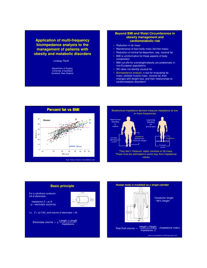
Percent fat vs BMI
Rush, Freitas, Plank Br J Nutr 2009;102: 632
Women
BMI, kg/m2 15 20 25 30 35 40 45 50 Body fat, % 10 20 30 40 50 60
AI E PI M
Percent fat vs BMI
Obese
Impedance (derived from measured voltage)
~
Constant alternating current
Bioelectrical impedance devices measure impedance at one
- r more frequencies
They don’t ‘measure’ water volumes or fat mass. These must be estimated in some way from impedance values
Impedance Constant current
Hand-to-foot Standing
- r
supine Leg-to-leg Standing (or arm-to-arm)
Basic principle
For a cylindrical conductor full of electrolyte: Impedance Z = ρL/A (ρ = electrolyte resistivity) i.e, Z = ρL2/(AL) and volume of electrolyte = AL
Length x Length Impedance Electrolyte volume = ρ Height x Height Impedance, Z Total fluid volume ∝ (impedance index) Human body is modelled as a single cylinder Conductor length ~ 95% Height
Stahn et al Handbook of Anthropometry 2012