Announcements Monday, November 13 The third midterm is on this - PowerPoint PPT Presentation

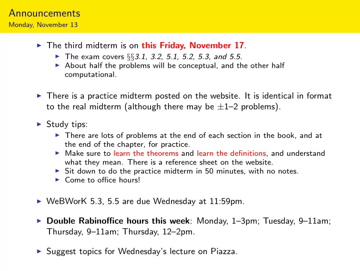
Announcements Monday, November 13 ◮ The third midterm is on this Friday, November 17 . ◮ The exam covers §§ 3.1, 3.2, 5.1, 5.2, 5.3, and 5.5. ◮ About half the problems will be conceptual, and the other half computational. ◮ There is a practice midterm posted on the website. It is identical in format to the real midterm (although there may be ± 1–2 problems). ◮ Study tips: ◮ There are lots of problems at the end of each section in the book, and at the end of the chapter, for practice. ◮ Make sure to learn the theorems and learn the definitions, and understand what they mean. There is a reference sheet on the website. ◮ Sit down to do the practice midterm in 50 minutes, with no notes. ◮ Come to office hours! ◮ WeBWorK 5.3, 5.5 are due Wednesday at 11:59pm. ◮ Double Rabinoffice hours this week : Monday, 1–3pm; Tuesday, 9–11am; Thursday, 9–11am; Thursday, 12–2pm. ◮ Suggest topics for Wednesday’s lecture on Piazza.

Geometric Interpretation of Complex Eigenvectors 2 × 2 case Theorem Let A be a 2 × 2 matrix with complex (non-real) eigenvalue λ , and let v be an eigenvector. Then A = PCP − 1 where � Re λ  | |  � Im λ P = Re v Im v and C = .   − Im λ Re λ | | The matrix C is a composition of rotation by − arg( λ ) and scaling by | λ | : � | λ | � � cos( − arg( λ )) � 0 − sin( − arg( λ )) C = . 0 | λ | sin( − arg( λ )) cos( − arg( λ )) A 2 × 2 matrix with complex eigenvalue λ is similar to (rotation by the argument of λ ) composed with (scaling by | λ | ). This is multiplication by λ in C ∼ R 2 .

Geometric Interpretation of Complex Eigenvalues 2 × 2 example � 1 − 1 � What does A = do geometrically? 1 1

Geometric Interpretation of Complex Eigenvalues 2 × 2 example, continued � 1 � − 1 A = C = λ = 1 − i 1 1 A rotate by π/ 4 √ scale by 2 [interactive]

Geometric Interpretation of Complex Eigenvalues Another 2 × 2 example � √ � 3 + 1 − 2 √ What does A = do geometrically? 1 3 − 1

Geometric Interpretation of Complex Eigenvalues Another 2 × 2 example, continued � √ � √ √ � � 3 + 1 − 2 3 − 1 √ √ A = C = λ = 3 − i 1 3 − 1 1 3

Geometric Interpretation of Complex Eigenvalues Another 2 × 2 example: picture � √ � 3 + 1 − 2 √ What does A = do geometrically? 1 3 − 1 C rotate by π/ 6 scale by 2 A = PCP − 1 does the same thing, but with respect to the basis �� 1 � − 1 � �� B = , of columns of P : 1 0 A “rotate around an ellipse” scale by 2 [interactive]

Classification of 2 × 2 Matrices with a Complex Eigenvalue Triptych Let A be a real matrix with a complex eigenvalue λ . One way to understand the geometry of A is to consider the difference equation v n +1 = Av n , i.e. the sequence of vectors v , Av , A 2 v , . . . � √ � √ � √ 1 3 + 1 − 2 � A = 1 � 1 3 + 1 − 2 � 3 + 1 − 2 √ √ A = √ √ A = √ 1 3 − 1 1 3 − 1 1 3 − 1 2 2 2 2 √ √ √ 3 − i 3 − i 3 − i λ = √ λ = √ λ = 2 2 2 2 | λ | = 1 | λ | > 1 | λ | < 1 v Av A 3 v A 2 v A 3 v A 2 v A 3 v Av v A 2 v Av v “spirals out” “rotates around an ellipse” “spirals in” [interactive] [interactive] [interactive]

Complex Versus Two Real Eigenvalues An analogy Theorem Let A be a 2 × 2 matrix with complex eigenvalue λ = a + bi (where b � = 0), and let v be an eigenvector. Then A = PCP − 1 where   | | P = Re v Im v and C = (rotation) · (scaling) .   | | This is very analogous to diagonalization. In the 2 × 2 case: Theorem Let A be a 2 × 2 matrix with linearly independent eigenvectors v 1 , v 2 and associated eigenvalues λ 1 , λ 2 . Then A = PDP − 1 scale x -axis by λ 1 scale y -axis by λ 2 where � λ 1   | | 0 � P = v 1 v 2 and D = .   0 λ 2 | |

Picture with 2 Real Eigenvalues We can draw analogous pictures for a matrix with 2 real eigenvalues. � 5 � Example: Let A = 1 3 . 3 5 4 This has eigenvalues λ 1 = 2 and λ 2 = 1 2 , with eigenvectors � 1 � � − 1 � v 1 = and v 2 = . 1 1 Therefore, A = PDP − 1 with � 1 � 2 � � − 1 0 P = and D = . 1 1 1 0 2 So A scales the v 1 -direction by 2 and the v 2 -direction by 1 2 . v 2 v 1 A v 2 v 1 scale v 1 by 2 scale v 2 by 1 2

Picture with 2 Real Eigenvalues We can also draw a picture from the perspective a difference equation: in other words, we draw v , Av , A 2 v , . . . � 5 λ 2 = 1 λ 1 = 2 A = 1 � 3 2 3 5 4 | λ 1 | > 1 | λ 1 | < 1 A 3 v v A 2 v Av v 2 v 1 [interactive] Exercise: Draw analogous pictures when | λ 1 | , | λ 2 | are any combination of < 1 , = 1 , > 1.

The Higher-Dimensional Case Theorem Let A be a real n × n matrix. Suppose that for each (real or complex) eigenvalue, the dimension of the eigenspace equals the algebraic multiplicity. Then A = PCP − 1 , where P and C are as follows: 1. C is block diagonal , where the blocks are 1 × 1 blocks containing the real eigenvalues (with their multiplicities), or 2 × 2 blocks containing the � Re λ � Im λ matrices for each non-real eigenvalue λ (with − Im λ Re λ multiplicity). 2. The columns of P form bases for the eigenspaces for the real eigenvectors, or come in pairs ( Re v Im v ) for the non-real eigenvectors. For instance, if A is a 3 × 3 matrix with one real eigenvalue λ 1 with eigenvector v 1 , and one conjugate pair of complex eigenvalues λ 2 , λ 2 with eigenvectors v 2 , v 2 , then     | | | λ 1 0 0 P = v 1 Re v 2 Im v 2 C = 0 Re λ 2 Im λ 2     | | | 0 − Im λ 2 Re λ 2

The Higher-Dimensional Case Example  1 − 1 0  Let A = 1 1 0  . This acts on the xy -plane by rotation by π/ 4 and  0 0 2 √ scaling by 2. This acts on the z -axis by scaling by 2. Pictures: from above looking down y -axis z z x x x y y [interactive] Remember, in general A = PCP − 1 is only similar to such a matrix C : so the x , y , z axes have to be replaced by the columns of P .

Summary ◮ There is a procedure analogous to diagonalization for matrices with complex eigenvalues. In the 2 × 2 case, the result is A = PCP − 1 where C is a rotation-scaling matrix. ◮ Multiplication by a 2 × 2 matrix with a complex eigenvalue λ spirals out if | λ | > 1, rotates around an ellipse if | λ | = 1, and spirals in if | λ | < 1. ◮ There are analogous pictures for 2 × 2 matrices with real eigenvalues. ◮ For larger matrices, you have to combine diagonalization and “complex diagonalization”. You get a block diagonal matrix with scalars and rotation-scaling matrices on the diagonal.