Announcements Reading for this lecture: Chapter 8. CSE 332: - - PDF document

1 CSE 332: Disjoint Set Union/Find (and finishing Dijkstra’s algorithm)

Richard Anderson, Steve Seitz Winter 2014

2

Announcements

• Reading for this lecture: Chapter 8.

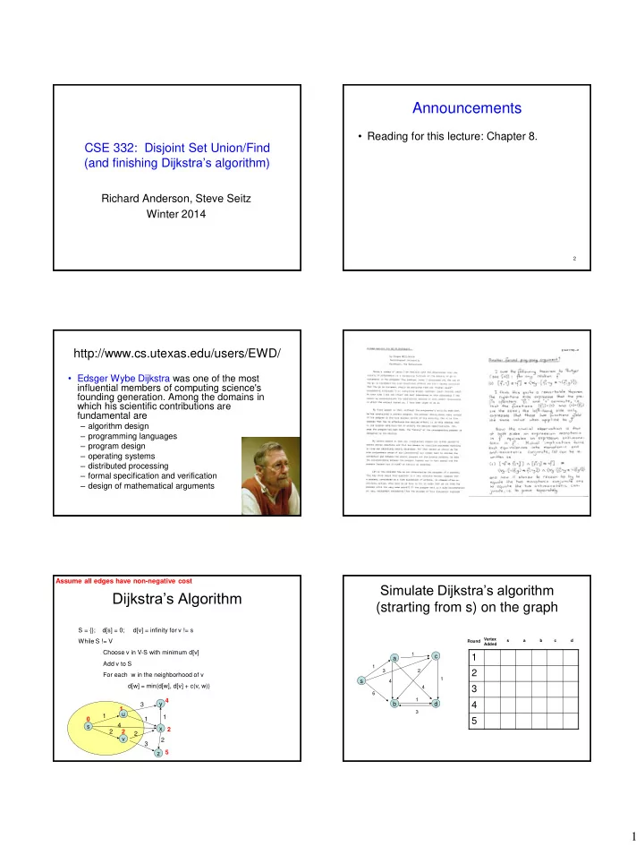
http://www.cs.utexas.edu/users/EWD/

• Edsger Wybe Dijkstra was one of the most

influential members of computing science's founding generation. Among the domains in which his scientific contributions are fundamental are

– algorithm design – programming languages – program design – operating systems – distributed processing – formal specification and verification – design of mathematical arguments

Dijkstra’s Algorithm

S = {}; d[s] = 0; d[v] = infinity for v != s While S != V Choose v in V-S with minimum d[v] Add v to S For each w in the neighborhood of v d[w] = min(d[w], d[v] + c(v, w)) s u v z y x 1 4 3 2 3 2 1 2 1 1 2 2 5 4

Assume all edges have non-negative cost

Simulate Dijkstra’s algorithm (strarting from s) on the graph

1 2 3 4 5

Round Vertex Added s a b c d

b d c a

1 1 1 2 3 4 6 1 3 4

s

2

Correctness Proof

• Elements in S have the correct label
• Key to proof: when v is added to S, it has

the correct distance label.

s y v x u

Proof

• Let v be a vertex in V-S with minimum d[v]
• Let Pv be a path of length d[v], with an edge (u,v)
• Let P be some other path to v. Suppose P first

leaves S on the edge (x, y)

– P = Psx + c(x,y) + Pyv – Len(Psx) + c(x,y) >= d[y] – Len(Pyv) >= 0 – Len(P) >= d[y] + 0 >= d[v]

s y v x u

Union-Find Data Structure

• ADT Definition
• How it’s implemented with pointers
• Optimizations
• Results of analysis

– (Some of the strangest mathematics in CS)

10

Making Connections

You have a set of nodes (numbered 1-9) on a network. You are given a sequence of pairwise connections between them: 3-5 4-2 1-6 5-7 4-8 3-7 Q: Are nodes 2 and 4 (indirectly) connected? Q: How about nodes 3 and 8? Q: Are any of the paired connections redundant due to indirect connections? Q: How many sub-networks do you have?

11

Making Connections

Answering these questions is much easier if we create disjoint sets of nodes that are connected: Start: {1} {2} {3} {4} {5} {6} {7} {8} {9} 3-5 4-2 1-6 5-7 4-8 3-7 Q: Are nodes 2 and 4 (indirectly) connected? Q: How about nodes 3 and 8? Q: Are any of the paired connections redundant due to indirect connections? Q: How many sub-networks do you have?

12

Applications of Disjoint Sets

Maintaining disjoint sets in this manner arises in a number of areas, including:

–Networks –Transistor interconnects –Compilers –Image segmentation –Building mazes (this lecture) –Graph problems

• Minimum Spanning Trees (upcoming topic in

this class)

3

13

Disjoint Set ADT

• Data: set of pairwise disjoint sets.
• Required operations

– Union – merge two sets to create their union – Find – determine which set an item appears in

• A common operation sequence:

– Connect two elements if not already connected: if (Find(x) != Find(y)) then Union(x,y)

14

Disjoint Sets and Naming

• Maintain a set of pairwise disjoint sets.

– {3,5,7} , {4,2,8}, {9}, {1,6}

• Each set has a unique name: one of its

members (for convenience)

– {3,5,7} , {4,2,8}, {9}, {1,6}

15

Union

• Union(x,y) – take the union of two sets

named x and y

– {3,5,7} , {4,2,8}, {9}, {1,6} – Union(5,1) {3,5,7,1,6}, {4,2,8}, {9},

16

Find

• Find(x) – return the name of the set

containing x.

– {3,5,7,1,6}, {4,2,8}, {9}, – Find(1) = 5 – Find(4) = 8

17

Example

S {1,2,7,8,9,13,19} {3} {4} {5} {6} {10} {11,17} {12} {14,20,26,27} {15,16,21} . . {22,23,24,29,39,32 33,34,35,36} Find(8) = 7 Find(14) = 20 S {1,2,7,8,9,13,19,14,20 26,27} {3} {4} {5} {6} {10} {11,17} {12} {15,16,21} . . {22,23,24,29,39,32 33,34,35,36} Union(7,20)

18

Nifty Application: Building Mazes

Idea: Build a random maze by erasing walls.

4

19

Building Mazes

• Pick Start and End

Start End

20

Building Mazes

• Repeatedly pick random walls to delete.

Start End

21

Desired Properties

• None of the boundary is deleted (except at

“start” and “end”).

• Every cell is reachable from every other cell.
• There are no cycles – no cell can reach itself by

a path unless it retraces some part of the path.

22

A Cycle

Start End

23

A Good Solution

Start End

24

A Hidden Tree

Start End

5

25

Number the Cells

Start End 1 2 3 4 5 6 7 8 9 10 11 12 13 14 15 16 17 18 19 20 21 22 23 24 25 26 27 28 29 30 31 32 33 34 35 36

We start with disjoint sets S ={ {1}, {2}, {3}, {4},… {36} }. We have all possible walls between neighbors W ={ (1,2), (1,7), (2,8), (2,3), … } 60 walls total. Idea: Union-find operations will be done on cells.

26

Maze Building with Disjoint Union/Find

Algorithm sketch:

• 1. Choose wall at random.

→ Boundary walls are not in wall list, so left alone

• 2. Erase wall if the neighbors are in disjoint sets.

→ Avoids cycles

• 3. Take union of those sets.
• 4. Go to 1, iterate until there is only one set.

→ Every cell reachable from every other cell.

27

Pseudocode

• S = set of sets of connected cells

– Initialize to {{1}, {2}, …, {n}}

• W = set of walls

– Initialize to set of all walls {{1,2},{1,7}, …}

• Maze = set of walls in maze (initially empty)

While there is more than one set in S Pick a random non-boundary wall (x,y) and remove from W u = Find(x); v = Find(y); if u  v then Union(u,v) else Add wall (x,y) to Maze Add remaining members of W to Maze

28

Example Step

Start End 1 2 3 4 5 6 7 8 9 10 11 12 13 14 15 16 17 18 19 20 21 22 23 24 25 26 27 28 29 30 31 32 33 34 35 36 S {1,2,7,8,9,13,19} {3} {4} {5} {6} {10} {11,17} {12} {14,20,26,27} {15,16,21} . . {22,23,24,29,30,32 33,34,35,36} Pick (8,14)

29

Example

S {1,2,7,8,9,13,19} {3} {4} {5} {6} {10} {11,17} {12} {14,20,26,27} {15,16,21} . . {22,23,24,29,39,32 33,34,35,36} Find(8) = 7 Find(14) = 20 S {1,2,7,8,9,13,19,14,20 26,27} {3} {4} {5} {6} {10} {11,17} {12} {15,16,21} . . {22,23,24,29,39,32 33,34,35,36} Union(7,20)

30

Example

Start End 1 2 3 4 5 6 7 8 9 10 11 12 13 14 15 16 17 18 19 20 21 22 23 24 25 26 27 28 29 30 31 32 33 34 35 36 S {1,2,7,8,9,13,19 14,20,26,27} {3} {4} {5} {6} {10} {11,17} {12} {15,16,21} . . {22,23,24,29,39,32 33,34,35,36} Pick (19,20)

6

31

Example at the End

Start End 1 2 3 4 5 6 7 8 9 10 11 12 13 14 15 16 17 18 19 20 21 22 23 24 25 26 27 28 29 30 31 32 33 34 35 36 S {1,2,3,4,5,6,7,… 36} Remaining walls in W Previously added to Maze

32

Data structure for disjoint sets?

• Represent: {3,5,7} , {4,2,8}, {9}, {1,6}
• Support: find(x), union(x,y)

33

Union/Find Trade-off

• Known result:

– Find and Union cannot both be done in worst- case O(1) time with any data structure.

• We will instead aim for good amortized

complexity.

• For m operations on n elements:

– Target complexity: O(m) i.e. O(1) amortized

34

Tree-based Approach

Each set is a tree

• Root of each tree is the set name.
• Allow large fanout (why?)

35

Up-Tree for DS Union/Find

1 2 3 4 5 6 7 Initial state 1 2 3 4 5 6 7 Intermediate state Roots are the names of each set. Observation: we will only traverse these trees upward from any given node to find the root. Idea: reverse the pointers (make them point up from child to parent). The result is an up-tree.

36

Find Operation

Find(x) follow x to the root and return the root.

1 2 3 4 5 6 7

7

37

Union Operation

Union(i, j) - assuming i and j roots, point i to j.

1 2 3 4 5 6 7

38

Simple Implementation

• Array of indices

1 2 3 4 5 6 7

1 2 3 4 5 6 7 up

up[x] = -1 means x is a root.

39

Implementation

int Find(int x) { while(up[x] >= 0) { x = up[x]; } return x; } void Union(int x, int y) { assert(up[x]<0 && up[y]<0); up[x] = y; }

runtime for Union: runtime for Find: Amortized complexity is no better.

40

A Bad Case

1 2 3 n

…

1 2 3 n Union(1,2) 1 2 3 n Union(2,3) Union(n-1,n)

… …

1 2 3 n

: : Find(1) n steps!!

41 42

Two Big Improvements

Can we do better? Yes!

• 1. Union-by-size
• Improve Union so that Find only takes worst

case time of Θ(log n).

• 2. Path compression
• Improve Find so that, with Union-by-size,

Find takes amortized time of almost Θ(1).

8

43

Union-by-Size

Union-by-size

– Always point the smaller tree to the root of the larger tree

1 2 3 4 5 6 7 S-Union(7,1) 2 4 1

44

Example Again

1 2 3 n 1 2 3 n S-Union(1,2) 1 2 3 n

S-Union(2,3) S-Union(n-1,n)

… …

: :

1 2 3 n

…

Find(1) constant time

…

45

Analysis of Union-by-Size

• Theorem: With union-by-size an up-tree of height h has size

at least 2h.

• Proof by induction

– Base case: h = 0. The up-tree has one node, 20 = 1 – Inductive hypothesis: Assume true for h-1 – Observation: tree gets taller only as a result of a union. h-1 T1 T2 T = S-Union(T1,T2) ≤h-1

46

Analysis of Union-by-Size

• What is worst case complexity of Find(x) in

an up-tree forest of n nodes?

• (Amortized complexity is no better.)

47

Worst Case for Union-by-Size

n/2 Unions-by-size n/4 Unions-by-size

48

Example of Worst Cast (cont’)

After n -1 = n/2 + n/4 + …+ 1 Unions-by-size Find If there are n = 2k nodes then the longest path from leaf to root has length k.

log2n

9

49

Array Implementation

1 2 3 4 5 6 7

• 1

2 1 -1 1 7 7 5 -1 4 1 2 3 4 5 6 7 up size Can store separate size array: 2 4 1

50

Elegant Array Implementation

1 2 3 4 5 6 7

• 2 1 -1 7 7 5 -4

1 2 3 4 5 6 7 up Better, store sizes in the up array: Negative up-values correspond to sizes of roots. 2 4 1

51

Code for Union-by-Size

S-Union(i,j){ // Collect sizes si = -up[i]; sj = -up[j]; // verify i and j are roots assert(si >=0 && sj >=0) // point smaller sized tree to // root of larger, update size if (si < sj) { up[i] = j; up[j] = -(si + sj); else { up[j] = i; up[i] = -(si + sj); } }

52

Path Compression

• To improve the amortized complexity, we’ll borrow an idea

from splay trees: – When going up the tree, improve nodes on the path!

• On a Find operation point all the nodes on the search path

directly to the root. This is called “path compression.” 1 2 3 4 5 6 7 1 2 3 4 5 6 7

PC-Find(3)

8 9 10 8 9 10

53

Self-Adjustment Works

PC-Find(x) x

54

Draw the result of Find(5):

6 8 1 2 3 4 5 7 9

10

55

Code for Path Compression Find

PC-Find(i) { //find root j = i; while (up[j] >= 0) { j = up[j]; root = j; //compress path if (i != root) { parent = up[i]; while (parent != root) { up[i] = root; i = parent; parent = up[parent]; } } return(root) }

56

• Worst case time complexity for…

– …a single Union-by-size is: – …a single PC-Find is:

• Time complexity for m  n operations on n

elements has been shown to be O(m log* n). [See Weiss for proof.] – Amortized complexity is then O(log* n) – What is log* ?

Complexity of Union-by-Size + Path Compression

57

log* n

log* n = number of times you need to apply log to bring value down to at most 1 log* 2 = 1 log* 4 = log* 22 = 2 log* 16 = log* 222 = 3 (log log log 16 = 1) log* 65536 = log* 2222 = 4 (log log log log 65536 = 1) log* 265536 = …………… ≈ log* (2 x 1019,728) = 5 log * n ≤ 5 for all reasonable n.

58

The Tight Bound

In fact, Tarjan showed the time complexity for m  n operations on n elements is: Q(m a(m, n)) Amortized complexity is then Q(a(m, n)) . What is a(m, n)? – Inverse of Ackermann’s function. – For reasonable values of m, n, grows even slower than log * n. So, it’s even “more constant.” Proof is beyond scope of this class. A simple algorithm can lead to incredibly hardcore analysis!