Announcements U 4: I - - PowerPoint PPT Presentation

U 4: I    L 4: ANOVA S 101

Nicole Dalzell June 3, 2015

Announcements

Announcements

If I still have your midterm, pick it up at the end of class. Lab 5 Today Office Hours Tomorrow Project Changes

Statistics 101 (Nicole Dalzell) U4 - L4: ANOVA June 3, 2015 2 / 40 ANOVA Classy vocabulary

The GSS gives the following 10 question vocabulary test:

A SPACE (school, noon, captain, room, board, don’t know) B BROADEN (efface, make level, elapse, embroider, widen, don’t know) C EMANATE (populate, free, prominent, rival, come, don’t know) D EDIBLE (auspicious, eligible, fit to eat, sagacious, able to speak, don’t know) E ANIMOSITY (hatred, animation, disobedience, diversity, friendship, don’t know) F PACT (puissance, remonstrance, agreement, skillet, pressure, don’t know) G CLOISTERED (miniature, bunched, arched, malady, secluded, don’t know) H CAPRICE (value, a star, grimace, whim, inducement, don’t know) I ACCUSTOM (disappoint, customary, encounter, get used to, business, don’t know) J ALLUSION (reference, dream, eulogy, illusion, aria, don’t know)

vocabulary scores

2 4 6 8 10 100 200

Statistics 101 (Nicole Dalzell) U4 - L4: ANOVA June 3, 2015 3 / 40 ANOVA Classy vocabulary

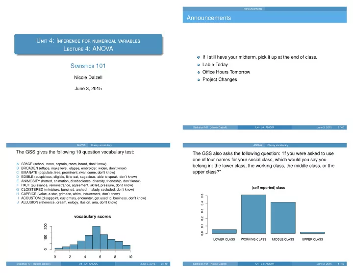
The GSS also asks the following question: “If you were asked to use

• ne of four names for your social class, which would you say you

belong in: the lower class, the working class, the middle class, or the upper class?”

LOWER CLASS WORKING CLASS MIDDLE CLASS UPPER CLASS

(self reported) class

0.0 0.1 0.2 0.3 0.4 0.5

Statistics 101 (Nicole Dalzell) U4 - L4: ANOVA June 3, 2015 4 / 40

ANOVA Classy vocabulary

Data

wordsum class 1 6 MIDDLE CLASS 2 9 WORKING CLASS 3 6 WORKING CLASS 4 5 WORKING CLASS 5 6 WORKING CLASS 6 6 WORKING CLASS 7 8 MIDDLE CLASS 8 10 WORKING CLASS 9 8 WORKING CLASS 10 9 UPPER CLASS

· · ·

795 9 MIDDLE CLASS

Statistics 101 (Nicole Dalzell) U4 - L4: ANOVA June 3, 2015 5 / 40 ANOVA Classy vocabulary

Exploratory analysis

• LOWER CLASS

WORKING CLASS MIDDLE CLASS UPPER CLASS 2 4 6 8 10

n mean sd lower class 41 5.07 2.24 working class 407 5.75 1.87 middle class 331 6.76 1.89 upper class 16 6.19 2.34

• verall

795 6.14 1.98

Statistics 101 (Nicole Dalzell) U4 - L4: ANOVA June 3, 2015 6 / 40 ANOVA ANOVA and the F test

Participation question Which of the following plots shows groups with means that are most and least likely to be significantly different from each other?

• 5

10 15 20 25 30 35

I

• −5

5 10 15 20

II

• −5

5 10 15 20 25

III

(a) most: I, least: II (b) most: II, least: III (c) most: I, least: III (d) most: III, least: II (e) most: II, least: I

Statistics 101 (Nicole Dalzell) U4 - L4: ANOVA June 3, 2015 7 / 40 ANOVA ANOVA and the F test

Step 2: Hypotheses

Is there a difference between the average vocabulary scores of Amer- icans from different (self reported) classes? H0 : The mean outcome is the same across all categories,

µLC = µWC = µMC = µUC

where µi represents the mean of the outcome for observations in category i. HA : At least one pair of means are different from each other.

Statistics 101 (Nicole Dalzell) U4 - L4: ANOVA June 3, 2015 8 / 40

ANOVA ANOVA and the F test

More generally...

H0 : The mean outcome is the same across all categories,

µ1 = µ2 = · · · = µk,

where µi represents the mean of the outcome for observations in category i. HA : At least one pair of means are different from each other.

Statistics 101 (Nicole Dalzell) U4 - L4: ANOVA June 3, 2015 9 / 40 ANOVA ANOVA and the F test

z/t test vs. ANOVA - Purpose

z/t test Compare means from two groups to see whether they are so far apart that the observed difference cannot reasonably be attributed to sampling variability. H0 : µ1 = µ2 ANOVA Compare the means from two or more groups to see whether they are so far apart that the observed differences cannot all reasonably be attributed to sampling variability. H0 : µ1 = µ2 = · · · = µk

Statistics 101 (Nicole Dalzell) U4 - L4: ANOVA June 3, 2015 10 / 40 ANOVA ANOVA and the F test

How do we compare multiple groups?

SST = SSG + SSE

Statistics 101 (Nicole Dalzell) U4 - L4: ANOVA June 3, 2015 11 / 40 ANOVA ANOVA and the F test

How do we compare multiple groups?

Sum of squares total, SST

Measures the total variability in the data SST =

n

• i=1

(xi − ¯

x)2 where xi represent the value of the response variable of each observation in the dataset.

Sum of squares between groups, SSG

Measures the variability between groups, i.e. how the group means com- pare to the grand mean SSG =

k

• j=1

ni(¯ xj − ¯ x)2 nj: each group size, ¯ xj: average for each group, ¯ x: overall (grand) mean

[Explained variability: deviation of group mean from overall mean, weighted by sample size.]

Statistics 101 (Nicole Dalzell) U4 - L4: ANOVA June 3, 2015 12 / 40

ANOVA ANOVA and the F test

Building the Test Statistic

SST = SSG + SSE If a group mean is very different from another is SSG large or small ? Since SST, the total sum of squares, is constant, what happens to SSE when SSG is large? So, when the SSG is large, what happens to the ratio SSG/SSE?

Statistics 101 (Nicole Dalzell) U4 - L4: ANOVA June 3, 2015 13 / 40 ANOVA ANOVA and the F test

Introducing the Mean Square

SSG SSE This ratio is large when putting the data into their groups seems to help us explain some of the variability in our data, ie when at least one group mean is dfiferent enough from the rest that we need to take notice. So, can we use this as our test statistic?? not quite Why not?? Splitting the data into groups means that the amount of data we are using to estimate each group mean goes down. We have to account for this somehow in the ratio in order for us to be able to use it as a test statistic.

Statistics 101 (Nicole Dalzell) U4 - L4: ANOVA June 3, 2015 14 / 40 ANOVA ANOVA and the F test

Mean Square

MSG is mean square between groups MSG = SSG dfG

= SSG

k − 1 where k is number of groups MSE is mean square error - variability in residuals MSE = SSE dfE

= SSE

n − k where n is number of observations.

Statistics 101 (Nicole Dalzell) U4 - L4: ANOVA June 3, 2015 15 / 40 ANOVA ANOVA and the F test

Test statistic

F = variability bet. groups variability w/in groups = MSG MSE MSG is mean square between groups MSG = SSG dfG

= SSG

k − 1 where k is number of groups MSE is mean square error - variability in residuals MSE = SSE dfE

= SSE

n − k where n is number of observations.

Statistics 101 (Nicole Dalzell) U4 - L4: ANOVA June 3, 2015 16 / 40

ANOVA ANOVA and the F test

Step 4: Picture of our Null Universe

F = variability bet. groups variability w/in groups F = MSG/MSE = 78.855/3.628 ≈ 21.735

Statistics 101 (Nicole Dalzell) U4 - L4: ANOVA June 3, 2015 17 / 40 ANOVA ANOVA and the F test

Step 4: Picture of our Null Universe

F = variability bet. groups variability w/in groups F = MSG/MSE = 78.855/3.628 ≈ 21.735 In order to be able to reject H0, we need a small p-value, which requires a large F statistic. In order to obtain a large F statistic, variability between sample means needs to be greater than variability within sample means.

Statistics 101 (Nicole Dalzell) U4 - L4: ANOVA June 3, 2015 18 / 40 ANOVA ANOVA and the F test

Test statistic

Can we see this in the boxplot?

• LOWER CLASS

WORKING CLASS MIDDLE CLASS UPPER CLASS 2 4 6 8 10

Does there appear to be a lot of variability within self-reported classes? How about between or across the classes?

Statistics 101 (Nicole Dalzell) U4 - L4: ANOVA June 3, 2015 19 / 40 ANOVA ANOVA and the F test

Step 5: Compute our P-value

F = variability bet. groups variability w/in groups P(F ≥ 21.735) < 0.0001 Note that you will need access to R to calculate the p-value. You can use the following function:

> pf(F-score, df_group, df_error, lower.tail = FALSE)

Statistics 101 (Nicole Dalzell) U4 - L4: ANOVA June 3, 2015 20 / 40

ANOVA ANOVA and the F test

Application exercise: ANOVA output The data provide convincing evidence that the: (a) average vocabulary scores are different for all classes. (b) average vocabulary score for middle class is higher than the average for the lower class. (c) average vocabulary score is different for at least one pair of classes. (d) average vocabulary scores are the same for all classes. (e) average vocabulary scores are different for upper and lower classes.

Statistics 101 (Nicole Dalzell) U4 - L4: ANOVA June 3, 2015 21 / 40 ANOVA ANOVA output, deconstructed

Df Sum Sq Mean Sq F value Pr(>F) (Group) class 3 236.56 78.855 21.735 <0.0001 (Error) Residuals 791 2869.80 3.628 Total 794 3106.36

Sum of squares total, SST Measures the total variability in the data SST =

n

• i=1

(xi − ¯

x)2 where xi represent the value of the response variable of each obser- vation in the dataset.

[Very similar to calculation of variance, except not scaled by the sample size.]

SST

= (6 − 6.14)2 + (9 − 6.14)2 + · · · + (9 − 6.14)2 =

3106.36

Statistics 101 (Nicole Dalzell) U4 - L4: ANOVA June 3, 2015 22 / 40 ANOVA ANOVA output, deconstructed

Df Sum Sq Mean Sq F value Pr(>F) (Group) class 3 236.56 78.855 21.735 <0.0001 (Error) Residuals 791 2869.80 3.628 Total 794 3106.36

Sum of squares between groups, SSG Measures the variability between groups, i.e. how the group means compare to the grand mean SSG =

k

• j=1

ni(¯ xj − ¯ x)2 nj: each group size, ¯ xj: average for each group, ¯ x: overall (grand) mean

[Explained variability: deviation of group mean from overall mean, weighted by sample size.]

n mean sd lower class 41 5.07 2.24 working class 407 5.75 1.87 middle class 331 6.76 1.89 upper class 16 6.19 2.34

• verall

795 6.14 1.98 SSG =

• 41 × (5.07 − 6.14)2

+

• 407 × (5.75 − 6.14)2

+

• 331 × (6.76 − 6.14)2

+

• 16 × (6.19 − 6.14)2

= 236.56

Statistics 101 (Nicole Dalzell) U4 - L4: ANOVA June 3, 2015 23 / 40 ANOVA ANOVA output, deconstructed

Df Sum Sq Mean Sq F value Pr(>F) (Group) class 3 236.56 78.855 21.735 <0.0001 (Error) Residuals 791 2869.80 3.628 Total 794 3106.36

Sum of squares error, SSE Measures the variability within groups: SSE = SST − SSG

[Unexplained variability, i.e. unexplained by the group variable, due to other reasons]

SSE = 3106.36 − 236.56 = 2869.80

Statistics 101 (Nicole Dalzell) U4 - L4: ANOVA June 3, 2015 24 / 40

ANOVA ANOVA output, deconstructed

now we need a way to get from these measures of total variability to average variability (scaling by a measure that incorporates sample sizes and number of groups → degrees of freedom)

Df Sum Sq Mean Sq F value Pr(>F) (Group) class 3 236.56 78.855 21.735 <0.0001 (Error) Residuals 791 2869.80 3.628 Total 794 3106.36

Statistics 101 (Nicole Dalzell) U4 - L4: ANOVA June 3, 2015 25 / 40 ANOVA ANOVA output, deconstructed

now we need a way to get from these measures of total variability to average variability (scaling by a measure that incorporates sample sizes and number of groups → degrees of freedom)

Df Sum Sq Mean Sq F value Pr(>F) (Group) class 3 236.56 78.855 21.735 <0.0001 (Error) Residuals 791 2869.80 3.628 Total 794 3106.36

The GROUP degrees of freedom dfG is the number of groups k minus 1. The TOTAL degrees of freedom df is n − 1. The ERROR degrees of freedom dfE is n − k df = dfG + dfE

Statistics 101 (Nicole Dalzell) U4 - L4: ANOVA June 3, 2015 26 / 40 ANOVA ANOVA output, deconstructed

Df Sum Sq Mean Sq F value Pr(>F) (Group) class 3 236.56 78.855 21.735 <0.0001 (Error) Residuals 791 2869.80 3.628 Total 794 3106.36

Mean squares Associated sum of squares divided by the associated df: MS = SS/df MSG = 236.56/3 = 78.855 MSE = 2869.80/791 = 3.628

Statistics 101 (Nicole Dalzell) U4 - L4: ANOVA June 3, 2015 27 / 40 ANOVA ANOVA output, deconstructed

Df Sum Sq Mean Sq F value Pr(>F) (Group) class 3 236.56 78.855 21.735 <0.0001 (Error) Residuals 791 2869.80 3.628 Total 794 3106.36

Test statistic, F value Ratio of the between group and within group variability: F = MSG

MSE

F = MSG/MSE = 78.855/3.628 ≈ 21.735

Statistics 101 (Nicole Dalzell) U4 - L4: ANOVA June 3, 2015 28 / 40

ANOVA ANOVA output, deconstructed

Solution

Statistics 101 (Nicole Dalzell) U4 - L4: ANOVA June 3, 2015 29 / 40 ANOVA Checking conditions

Checking Assumptions

We sort of blew through Step 3. Let’s go back to that...

Statistics 101 (Nicole Dalzell) U4 - L4: ANOVA June 3, 2015 30 / 40 ANOVA Checking conditions

(1) independence

If the data are a simple random sample from less than 10% of the population, this condition is satisfied. Carefully consider whether the data may be independent (e.g. no pairing). Always important, but sometimes difficult to check. Does this condition appear to be satisfied?

Statistics 101 (Nicole Dalzell) U4 - L4: ANOVA June 3, 2015 31 / 40 ANOVA Checking conditions

(2) approximately normal

The observations within each group should be nearly normal (especially important when the sample sizes are small.) Does this condition appear to be satisfied?

• LOWER CLASS

WORKING CLASS MIDDLE CLASS UPPER CLASS 2 4 6 8 10

Statistics 101 (Nicole Dalzell) U4 - L4: ANOVA June 3, 2015 32 / 40

ANOVA Checking conditions

(3) constant variance

The variability across the groups should be about equal (especially important when the sample sizes differ between groups.) Does this condition appear to be satisfied?

• LOWER CLASS

WORKING CLASS MIDDLE CLASS UPPER CLASS 2 4 6 8 10

n mean sd lower class 41 5.07 2.24 working class 407 5.75 1.87 middle class 331 6.76 1.89 upper class 16 6.19 2.34

Statistics 101 (Nicole Dalzell) U4 - L4: ANOVA June 3, 2015 33 / 40 ANOVA Checking conditions

Relevant formulas

Degrees of freedom associated with ANOVA groups: dfG = k − 1, where k is the number of groups total: dfT = n − 1, where n is the total sample size error: dfE = dfT − dfG Mean squares Associated sum of squares divided by the associated df: MS = SS/df Test statistic, F value Ratio of the between group and within group variability: F = MSG

MSE

p-value Probability of at least as large a ratio between the “between group” and “within group” variability as the one observed, if in fact the means of all groups are equal – calculated as the area under the F curve, with degrees of freedom dfG and dfE, above the observed F statistic.

Statistics 101 (Nicole Dalzell) U4 - L4: ANOVA June 3, 2015 34 / 40 Multiple comparisons & Type 1 error rate

Which means differ?

Earlier we concluded that at least one pair of means differ. The natural question that follows is “which ones?” We can do two sample t tests for differences in each possible pair of groups. Can you see any pitfalls with this approach? When we run too many tests, the Type 1 Error rate increases. This issue is resolved by using a modified significance level.

Statistics 101 (Nicole Dalzell) U4 - L4: ANOVA June 3, 2015 35 / 40 Multiple comparisons & Type 1 error rate

Multiple comparisons

The scenario of testing many pairs of groups is called multiple comparisons. The Bonferroni correction suggests that a more stringent significance level is more appropriate for these tests:

α⋆ = α/K

where K is the number of comparisons being considered. If there are k groups, then usually all possible pairs are compared and K = k(k−1)

2

.

Statistics 101 (Nicole Dalzell) U4 - L4: ANOVA June 3, 2015 36 / 40

Multiple comparisons & Type 1 error rate

Determining the modified α

Participation question In the aldrin data set depth has 3 levels: bottom, mid-depth, and sur-

• face. If α = 0.05, what should be the modified significance level for two

sample t tests for determining which pairs of groups have significantly different means? (a) α∗ = 0.05 (b) α∗ = 0.05/2 = 0.025 (c) α∗ = 0.05/4 = 0.0125 (d) α∗ = 0.05/6 = 0.0083

Statistics 101 (Nicole Dalzell) U4 - L4: ANOVA June 3, 2015 37 / 40 Multiple comparisons & Type 1 error rate

Which means differ?

Based on the box plots below, which means would you expect to be significantly different?

• LOWER CLASS

WORKING CLASS MIDDLE CLASS UPPER CLASS 2 4 6 8 10

Statistics 101 (Nicole Dalzell) U4 - L4: ANOVA June 3, 2015 38 / 40 Multiple comparisons & Type 1 error rate

Which means differ? (cont.)

When doing multiple comparisons after ANOVA, since the assumption of equal variability across groups must have been satisfied, we re-think how we measure the standard error and the degrees of freedom. For all comparisons, use a consistent SE

SE: calculate SE using spooled =

√

MSE instead of s1 and s2. SE =

• s2

1

n1

+

s2

2

n2

→ SE =

• MSE

n1

+ MSE

n2 df: use df = dfE from ANOVA instead of df calculated based on individual sample sizes n1 and n2. df = min(n1 − 1, n2 − 1) → df = dfE

Finally, compare the p-value of this test to the modified significance level (α⋆).

Statistics 101 (Nicole Dalzell) U4 - L4: ANOVA June 3, 2015 39 / 40 Multiple comparisons & Type 1 error rate

Is there a difference between the average vocabulary scores between middle and lower class Americans?

Statistics 101 (Nicole Dalzell) U4 - L4: ANOVA June 3, 2015 40 / 40