Announcements Homework 1 is due Apr 24, 11:59 PM Homework 2 will - - PDF document

announcements
SMART_READER_LITE
LIVE PREVIEW

Announcements Homework 1 is due Apr 24, 11:59 PM Homework 2 will - - PDF document

Announcements Homework 1 is due Apr 24, 11:59 PM Homework 2 will be assigned this week Reading: Binary Image Processing Chapter 3 Image processing Introduction to Computer Vision CSE 152 Lecture 8 CSE 152, Spring 2015


slide-1
SLIDE 1

1

CSE 152, Spring 2015 Introduction to Computer Vision

Binary Image Processing

Introduction to Computer Vision CSE 152 Lecture 8

CSE 152, Spring 2015 Introduction to Computer Vision

Announcements

  • Homework 1 is due Apr 24, 11:59 PM
  • Homework 2 will be assigned this week
  • Reading:

– Chapter 3 Image processing

CSE 152, Spring 2015 Introduction to Computer Vision

Binary System Summary

1. Acquire images and binarize (tresholding, color labels, etc.). 2. Possibly clean up image using morphological

  • perators.

3. Determine regions (blobs) using connected component exploration 4. Compute position, area, and orientation of each blob using moments 5. Compute features that are rotation, scale, and translation invariant using Moments (e.g., Eigenvalues of normalized moments).

CSE 152, Spring 2015 Introduction to Computer Vision

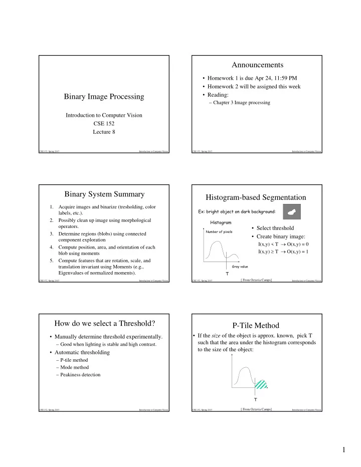
Histogram-based Segmentation

  • Select threshold
  • Create binary image:

I(x,y) < T  O(x,y) = 0 I(x,y)  T  O(x,y) = 1

Ex: bright object on dark background: T

Gray value Number of pixels

Histogram

[ From Octavia Camps]

CSE 152, Spring 2015 Introduction to Computer Vision

How do we select a Threshold?

  • Manually determine threshold experimentally.

– Good when lighting is stable and high contrast.

  • Automatic thresholding

– P-tile method – Mode method – Peakiness detection

CSE 152, Spring 2015 Introduction to Computer Vision

P-Tile Method

  • If the size of the object is approx. known, pick T

such that the area under the histogram corresponds to the size of the object:

T

[ From Octavia Camps]

slide-2
SLIDE 2

2

CSE 152, Spring 2015 Introduction to Computer Vision

Mode Method

  • Model intensity in each region Ri as

“constant” + N(0,i):

[ From Octavia Camps]

CSE 152, Spring 2015 Introduction to Computer Vision

Example: Image with 3 regions

Ideal histogram: 1 3 2 If above image is noisy, histogram looks like 1 3 2

  • Approximate histogram

as being comprised of multiple Gaussian modes.

  • How many modes?
  • Where are they

centered, width

  • Altenatively,the valleys

are good places for thresholding to separate regions.

[ From Octavia Camps]

CSE 152, Spring 2015 Introduction to Computer Vision

Finding the peaks and valleys

  • It is a not trivial problem:

[ From Octavia Camps]

CSE 152, Spring 2015 Introduction to Computer Vision

“Peakiness” Detection Algorithm

  • Find the two HIGHEST LOCAL MAXIMA that

MINIMUM DISTANCE APART: gi and gj

  • Find lowest point between them: gk
  • Measure “peakiness”:

– min(H(gi),H(gj))/H(gk)

  • Find (gi,gj,gk) with highest peakiness

gi gj gk

[ From Octavia Camps]

CSE 152, Spring 2015 Introduction to Computer Vision

Regions

CSE 152, Spring 2015 Introduction to Computer Vision

What is a region?

  • “Maximal connected set of points in the image

with same brightness value” (e.g., 1)

  • Two points are connected if there exists a

continuous path joining them.

  • Regions can be simply connected (For every pair
  • f points in the region, all smooth paths can be

smoothly and continuously deformed into each

  • ther). Otherwise, region is multiply connected

(holes)

slide-3
SLIDE 3

3

CSE 152, Spring 2015 Introduction to Computer Vision

Connected Regions

1 1 1 1 1 1 1 1 1 1 1 1 1 1 1 1 1 1 1 1 1 1 1 1 1 1 1 1 1 1

  • What are the connected regions in this binary image?
  • Which regions are contained within which region?

CSE 152, Spring 2015 Introduction to Computer Vision

Connected Regions

1 1 1 1 1 1 1 1 1 1 1 1 1 1 1 1 1 1 1 1 1 1 1

  • What the connected regions in this binary image?
  • Which regions are contained within which region?

CSE 152, Spring 2015 Introduction to Computer Vision

Four & Eight Connectedness

Eight Connected Four Connected

CSE 152, Spring 2015 Introduction to Computer Vision

Almost obvious

Jordan Curve Theorem

  • “Every closed curve in R2 divides the plane

into two region, the ‘outside’ and ‘inside’ of the curve.”

CSE 152, Spring 2015 Introduction to Computer Vision

Problem of 4/8 Connectedness

1 1 1 1 1 1 1 1 1 1

  • 8 Connected:

– 1’s form a closed curve, but background only forms one region.

  • 4 Connected

– Background has two regions, but ones form four “open” curves (no closed curve)

CSE 152, Spring 2015 Introduction to Computer Vision

To achieve consistency with respect to Jordan Curve Theorem

1. Treat background as 4-connected and foreground as 8-connected. 2. Use 6-connectedness

slide-4
SLIDE 4

4

CSE 152, Spring 2015 Introduction to Computer Vision

Recursive Labeling Connected Component Exploration

Procedure Label (Pixel) BEGIN Mark(Pixel) <- Marker; FOR neighbor in Neighbors(Pixel) DO IF Image (neighbor) = 1 AND Mark(neighbor)=NIL THEN Label(neighbor) END BEGIN Main Marker <- 0; FOR Pixel in Image DO IF Image(Pixel) = 1 AND Mark(Pixel)=NIL THEN BEGIN Marker <- Marker + 1; Label(Pixel); END; END Globals: Marker: integer Mark: Matrix same size as Image, initialized to NIL

CSE 152, Spring 2015 Introduction to Computer Vision

Recursive Labeling Connected Component Exploration

 

CSE 152, Spring 2015 Introduction to Computer Vision

Some notes

  • Once labeled, you know how many regions

(the value of Marker)

  • From Mark matrix, you can identify all

pixels that are part of each region (and compute area)

  • How deep does stack go?
  • Iterative algorithms
  • Parallel algorithms

CSE 152, Spring 2015 Introduction to Computer Vision

Properties extracted from binary image

  • A tree showing containment of regions
  • Properties of a region
  • 1. Genus – number of holes
  • 2. Centroid
  • 3. Area
  • 4. Perimeter
  • 5. Moments (e.g., measure of elongation)
  • 6. Number of “extrema” (indentations, bulges)
  • 7. Skeleton

CSE 152, Spring 2015 Introduction to Computer Vision

Moments

1 Given a pair of non-negative integers (j,k) the discrete (j,k)th moment of S is defined as: B(x,y)



 

n x m y k j jk

y x y x B M

1 1

) , (

  • Fast way to implement

computation over n by m image or window

  • One object

The region S is defined as:

B

CSE 152, Spring 2015 Introduction to Computer Vision

Moments: Area

1 Example:

Area of S

slide-5
SLIDE 5

5

CSE 152, Spring 2015 Introduction to Computer Vision

Moments: Centroid

1 Example:

Center of gravity (centroid, mean) of S

CSE 152, Spring 2015 Introduction to Computer Vision

Shape recognition by Moments

1 1

=

?

Recognition could be done by comparing moments However, moments Mjk are not invariant under:

  • Translation
  • Scaling
  • Rotation
  • Skewing

CSE 152, Spring 2015 Introduction to Computer Vision

Central Moments

1 Given a pair of non-negative integers (j,k) the central (j,k)th moment of S is given by: Or the central moments can be computed from precomputed regular moments

 jk  i m      

n1 j

m1 i

 j n       (x )(im)(y )( j n)Mmn

CSE 152, Spring 2015 Introduction to Computer Vision

Central Moments

1 1 Translation by T = (a,b) : Translation INVARIANT

CSE 152, Spring 2015 Introduction to Computer Vision

Normalized Moments

1 Given a pair of non-negative integers (j,k) the normalized (j,k)th moment of S is given by:

CSE 152, Spring 2015 Introduction to Computer Vision

Normalized Moments

1 1 Scaling by (a,c) and translating by T = (b,d) : Scaling and translation INVARIANT

slide-6
SLIDE 6

6

CSE 152, Spring 2015 Introduction to Computer Vision

Region orientation from Second Moment Matrix

1. Compute second centralized moment matrix

  • 1. Compute Eigenvectors of Moment Matrix to obtain orientation
  • 2. Eigenvalues are independent of orientation and translation

     

02 11 11 20

   

  • Symmetric, positive definite matrix
  • Positive Eigenvalues
  • Orthogonal Eigenvectors

CSE 152, Spring 2015 Introduction to Computer Vision

Binarization using Color

  • Object’s in robocup are

distinguished by color.

  • How do you binarize the

image so that pixels where ball is located are labeled with 1, and other locations are 0?

  • Let Cb=(r g b)T be the color
  • f the ball.

CSE 152, Spring 2015 Introduction to Computer Vision

Binarization using Color

  • Let c(u,v) be the color of pixel (u,v)
  • Simple method
  • Better alternative (why?)

– Convert c(u,v) to HSV space H(u,v), S(u,v) V(u,v) – Convert cb to HSV – Check that HS distance is less than threshold  and brightness (V) is greater than a treshold V> b(u,v)  1 if ||c(u,v)  cb ||

 

2  

  • therwise

    