Analysis of a Mountain Wave Event Observed in AIRS and ECMWF Joan - - PowerPoint PPT Presentation

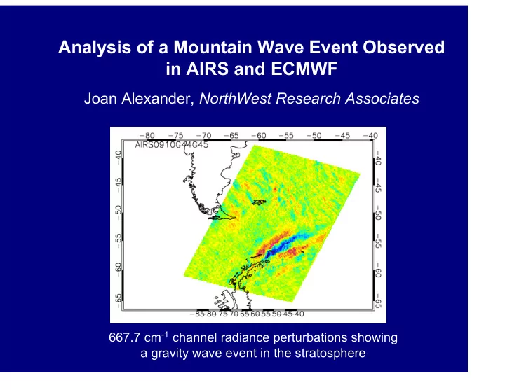
Analysis of a Mountain Wave Event Observed in AIRS and ECMWF

Joan Alexander, NorthWest Research Associates

667.7 cm-1 channel radiance perturbations showing a gravity wave event in the stratosphere

Global Effects on the Circulation Atmospheric Gravity Waves:

 Gravity waves are internal waves with small-scales compared to global.  They naturally grow in amplitude with height because of conservation of

energy and the exponential decrease in atmospheric density with height.

 They carry vertical flux of horizontal momentum through the atmosphere.  Upon breaking (dissipating), they drive large-scale circulations.

The Quasibiennial Oscillation (QBO) is a classic example of a wave-driven circulation. Roughly half of the wave momentum flux is carried by small-scale gravity waves.

Global Effects on the Circulation Atmospheric Gravity Waves:

 Mountain wave drag slows the winter jet in the upper troposphere and

stratosphere and helps to correct a “cold pole problem”.

 Currently treated via parameterization in climate and forecast models.  The wave momentum flux is dependent on sub-grid-scale topographic

variance, surface winds, stability, and tunable parameters.

Atmospheric Gravity Waves: Global Effects on Clouds and Chemistry

 The “cold pole problem” leads to

large errors in temperature-sensitive

• zone chemistry in the stratosphere.

 Gravity wave fluctuations can cause

polar stratospheric clouds to form in conditions that are otherwise too warm. Photo credit: Sean Dav Photo credit: Sean Dav PSCs over McMurdo, Antarctica PSCs over McMurdo, Antarctica

Parameterization of Mountain Wave Drag

(a forcing term for the RHS of the momentum equation)

• These determine the altitude where

the waves break or dissipate.

• 1-D Wave propagation is assumed

(vertical column calculation).

• The mean-flow force is proportional

to the vertical gradient of momentum flux and the force direction will always “drag” the mean-flow toward the wave phase speed.

• Mountain waves are stationary; they

therefore always act to slow the me flow speeds towards zero. Inputs:

• Wave momentum flux

(function of surface wind subgrid orography)

• Horizontal wavelength
• Wave phase speed =0
• Direction of propagation

(opposite surface wind)

• Background wind and

stability profiles

 Momentum Flux from Satellite Observations of Gravity Waves

 AIRS observes T' (temperature amplitude)  To convert to momentum flux, also need:

k = horizontal wavenumber m = vertical wavenumber φ = propagation direction Momentum Flux ~ (k/m) |T'/ T| 2

 For a given T', momentum flux will be larger for longer vertical

and shorter horizontal wavelength waves

 T' ( k,φ ) observed directly from AIRS high resolution images  For mountain waves, m = N/U (buoyancy frequency/wind speed)  For nonstationary waves, m must be computed from observations.

Effective Weighting Functions for gravity wave observations

(schematic)

• K

Sub-limb Viewing Limb Viewing Nadir Viewing

15 micron band 4.2 micron band

AIRS CO2 Temperature Sensing Channels Kernel Functions

 Gravity waves are detected in the AIRS temperature-sensing channels  Clouds interfere when weighting functions intersect cloud tops.

Alexander and Barnet [2007]

Mountain Wave Study: Distributions of Wave Properties from AIRS

Distribution of wave amplitudes and horizontal wavelengths derived from 40 radiance granules at 667.7 cm-1 in the stratosphere

• ver Patagonia and the Antarctic

Peninsula

 Peak amplitudes for horizontal

wavelengths of ~ 100 km.

 Loss of resolution in temperatur

retrievals (Δx ~ 20 km -> 60 km) is a severe drawback.

Vertical Wavelength Sensitivity

The depth of the weighting functions and the near-nadir view angles of AIRS mean there is little or no response to waves with vertical wavelengths less than 12 km.

Response vs Vertical Wavelength in the 15 µm band

667.77 cm-1 Channel Response

Case Study 10 September 2003 [Alexander & Teitelbaum, 2006]

 Large amplitude wave event near the Antarctic peninsula  Also seen in ECMWF forecast and assimilation fields

AIRS radiance at 667.7 cm-1 AIRS temperature retrieval at 40 km

 Radiances have Δx ~ 20 km  Retrievals have Δx ~ 60 km  The horizontal wavelength is 300 k

in the stratosphere, large enough to be resolved in the AIRS temperatur retrievals.

Case Study 10 September 2003

 Compare radiances and temperature retrievals to ECMWF  Focus on radiances because of higher horizontal resolution  For small perturbations, the Planck function gives:

Location of cross-sections viewed in the following slides

R'/R = T'/T (hcν/kT)

 Selecting 34 channels in the stratosphere and troposphere  Minimum height depends on cloud occurrence  Vertical binned average weighted by (channel noise)-1 = (neΔT)-1

Vertical gridding of radiances to create 3-d gravity wave images

Gridded product noise varies from K z 0.15-0.29 >30km 0.04 ~30km 0.09 <30km

Wave Event Vertical Cross-Sections

 The temperature retrieval sharpens vertical gradients. This

correctly increases the wave amplitude above ~30 km.

 The radiance response function predicts a wave response of ~1/3

for a 20-km vertical wavelength wave.

 Below 25-30 km, the waves have smaller horizontal scales that are

unresolved in the retrieval.

Cloud feature determined from auxiliary data

Wave Event Vertical Cross-Sections

 Comparison of AIRS retrieval and ECMWF shows remarkable similarity.  We use the time resolution of the ECMWF to study the origin of this

wave event.

0420 UT 0600 UT

• The ECMWF wave event has very similar scale and morphology.
• The perturbations appear directly above the peninsula at low altitude.
• At higher altitudes they appear north of the peninsula.

ECMWF Wind Divergence isolates the wave from the geostrophic mean flow

40 km 5 km

N N

ECMWF Wind Divergence at z=30 km three different times 00, 03, 06 UT

 The wave appears stationary relative to the peninsula topography  The event persists for at least 18 hours from ~12 UT on 9 Sept to ~18 UT on 10 Sept.  Stationarity of the wave event is consistent with a mountain wave interpretation.

00 06 03

ECMWF Surface Wind Vectors

 Low level winds blow

~ perpendicular to the Antarctic peninsula ridge.

 Optimal orientation

for large amplitude mountain wave forcing

Marambio (57oW, 64oS) Radiosonde Analysis

 Detrended vertical profiles  Two perpendicular components

(uR, vR) in coordinate system rotated by 80o from cardinal directions

 Angle chosen to maximize

the correlation coefficient between uR and vR

 Then uR, vR are in phase,

and the coordinate system is aligned with the propaga- tion direction of a medium frequency gravity wave

 This gives propagation direction

~opposite to the surface winds.

Background Wind Profiles and Theoretical Mountain Wave Vertical Wavelength

ECMWF and Radiosonde Wind Profiles Zonal Meridional Theoretical Vertical Wavelength Using the gravity wave dispersion relationship and winds in the mountain wave propagation direction:

λZ = N/(2π U) The observed vertical wavelength was 20 km at altitudes 40-43 km

Summary

 Analysis: AIRS radiance observations of a mountain wave event

Horizontal wavelength = 300 km Vertical wavelength = 20 km Propagation direction 40o west of north

 Vertical wavelength gives a radiance attenuation factor ~ 1/3

and estimated temperature amplitude ~ 10oK (12oK seen in the temperature retrieval)

 These allow estimation of the momentum flux using linear theory:

Momentum Flux ~ 1/2ρ(T'/T)2(k/m)(g/N)2

 AIRS provides the necessary information to constrain input

tuning parameters for gravity wave parameterizations.

 Note: 1-D propagation becomes a poor assumption as models

achieve higher horizontal resolution.