An introduction to R Rstudio is just a nice software A factor is - - PowerPoint PPT Presentation

An introduction to R

Jorge Cimentada and Basilio Moreno 6th of July 2019 Rstudio is just a nice software to run R! A factor is just a way of saying that a variable has unique values! And they can be ordered.

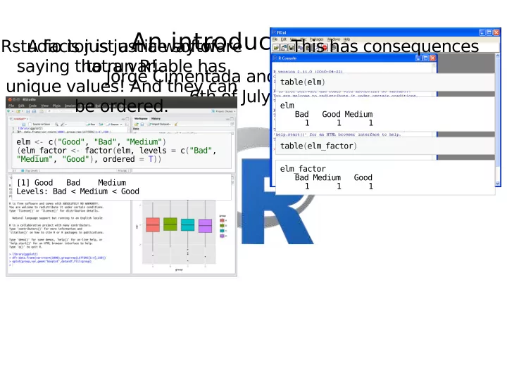
elm <- c("Good", "Bad", "Medium") (elm_factor <- factor(elm, levels = c("Bad", "Medium", "Good"), ordered = T)) [1] Good Bad Medium Levels: Bad < Medium < Good

This has consequences

table(elm) elm Bad Good Medium 1 1 1 table(elm_factor) elm_factor Bad Medium Good 1 1 1

How to install R?

Luckily, you guys have R and Rstudio installed, so you don't have to worry about this! But if you want to install it at home, please follow That guide can help you install

R Rstudio And swirl, a package in which you could do a bunch of exercises as homework!

this guide

What is R?

R is a programming language designed to do data analysis, usually interactive. R is helpful for..

Getting that darn excel/stata file into R (importing) Turning that very ugly dataset into something to work with (data cleaning) Automating your weekly reports (automating tasks) Analyzing data (modeling) Creating nicely formatted documents (communicating results) Building your own commands to do specific things (functions)

Building very creative graphics Among many things…

And so.. what is Rstudio?

And so.. what is Rstudio?

Let's get to it then!

R is an interactive language. That means that if you type a number, you will get a number.

#Input 10 [1] 10 #Input 5 [1] 5

Introduction to R objects

R is also a calculator Try typing these operations in R:

5 + 5 10 - 5 10 * 5 20 / 10 (10 * 20) - 5 / 2 + 2 2 ^ 3

Before we continue, what type of operations are these? Answers in next slide!

Introduction to R objects

Addition Subtraction Multiplication Division A combination of all Exponentiation

Numbers in R are called numerics. For example:

is.numeric(10) is.numeric(10 + 20) is.numeric(10 / 2)

Introduction to R objects

Having single numbers, like 10, is not very useful. We want something similar to a column of a dataset, like age or income. We can do that with c(), which stands for concatenate. Read this expression as: concatenate these numbers into a single object.

c(32, 34, 18, 22, 65) [1] 32 34 18 22 65

Introduction to R objects

We can also give it a name, like age.

Why didn't the result get printed? Where is this age object at? What is formally the age object?

age <- c(32, 34, 18, 22, 65)

Introduction to R objects

We just created our first variable! The typical SAS/Excel/Stata column. In R, these objects are called 'vectors'. Vectors can have several flavours:

Numerics (we just saw one) Logicals Characters Factors

Introduction to R objects

Suppose these ages belong to certain people. We can create a character vector with their names. Following this guideline, create it yourself.

Create a character vector with c() Include the names Paul, Maria, Andres, Roberto and Alicia inside wrap every name in quotes like this “Paul”, “Maria”, etc… This will make R understand that input as characters.

Introduction to R objects

Answer: We can also give it a name, like participants.

c("Paul", "Maria", "Andres", "Robert", "Alicia") [1] "Paul" "Maria" "Andres" "Robert" "Alicia" participants <- c("Paul", "Maria", "Andres", "Robert", "Alicia")

Introduction to R objects

Character vectors are filled by strings, like “Paul” or “Maria”. Can we do operations with strings? Makes sense.. we can't add any letters. Alright, we're set. Concatenate the numeric vector age and participants.

"Paul" + "Maria" Error in "Paul" + "Maria": non-numeric argument to binary operator

Introduction to R objects

What's the problem with this result?

c(age, participants) [1] "32" "34" "18" "22" "65" "Paul" "Maria" [8] "Andres" "Robert" "Alicia"

This breaks an R law!

We joined a numeric vector and a character vector. Vectors can ONLY be of one class.

c(1, "one") # forces to character vector [1] "1" "one" c(1, "1") # note that the first one is a numeric, while the second is a character [1] "1" "1"

Introduction to R objects

Now, which of these people has an age above 20?

That's a logical vector.

Contrary to character and numeric vectors, logical vectors can only have three values:

TRUE FALSE NA (which stands for “Not available”.)

age > 20 [1] TRUE TRUE FALSE TRUE TRUE

Introduction to R objects

logicals can be created manually or with a logical statement. The above expression tests for the logical statement. For example,

c(TRUE, FALSE, TRUE, TRUE) [1] TRUE FALSE TRUE TRUE age < 60 [1] TRUE TRUE TRUE TRUE FALSE 32 34 18 22 65 TRUE TRUE TRUE TRUE FALSE

Introduction to R objects

You can also write T or F as short abbreviations of TRUE and FALSE. Which is comparing: But behind the scenes, TRUE and T are just a 1 and F and FALSE are just a 0. What is the result of this?

c(T, T, F, T) == c(TRUE, TRUE, FALSE, TRUE) [1] TRUE TRUE TRUE TRUE TRUE TRUE FALSE TRUE "T" "T" "F" "T" T + 5 TRUE - 5 FALSE + TRUE T + T - FALSE

Introduction to R objects

Now that you know that.. what would be the class of the following vectors?

numeric: TRUE is coerced to 1 character: “FALSE” is a string, can't be turned to a number logical: both elements are logical! numeric: FALSE is coerced to 0

c(5, TRUE) c(5, "FALSE") c(FALSE, TRUE) c(1, FALSE)

Introduction to R objects

What do we know so far?

Numeric vectors Character vectors Logical vectors How to assign a name to these vectors Vectors can contain only one class of data

What's missing?

Factors

Introduction to R objects

Factors are R's way of storing categorical variables. Categories such as:

'Male' and 'Female' or 'Married' and 'Divorced' 'Good', 'Middle' and 'High'

gender <- c("Male", "Female", "Male", "Male", "Female") # Can be turned into gender <- factor(gender)

Introduction to R objects

Introduction to R objects

Factors are useful for some specific operations like:

Changing order of levels for terms in modelling Changing order of axis labels in plots Among other things..

In many cases you can use characters to do what you would want with factors!

Introduction to R objects

Now, have you noticed that we've been assigning names to things? The name age holds all these elements inside. How do we know where all the variables we've created are? Let's ask R what objects can be listed from our workspace or environment.

age [1] 32 34 18 22 65 ls() [1] "age" "elm" "elm_factor" "gender" [5] "lgl" "participants"

Introduction to R objects

So far, we have a bunch of variables scattered around

• ur workspace. This is usually no the way to go!

We want to group similar things in the same place.

A data frame is usually the primary structure of analysis in R

• ur_df <- data.frame(name = participants, age = age, gender = gender, age_60 = lgl)
• ur_df

name age gender age_60 1 Paul 32 Male TRUE 2 Maria 34 Female TRUE 3 Andres 18 Male TRUE 4 Robert 22 Male TRUE 5 Alicia 65 Female FALSE

Introduction to R objects

It's important that you understand the thing that defines a data frame.

A data frame has rows and columns, more technically called dimensions. Data frames have two dimensions.

dim(our_df) [1] 5 4 nrow(our_df) [1] 5 ncol(our_df) [1] 4

Introduction to R objects

Data frames are very distinctive because they can hold any type of vector. Matrices cannot!

Matrices are very similar to data frames. They have same number of dimensions. You can choose rows/columns in similar ways.

• ur_matrix <- matrix(1:20, ncol = 4, nrow = 5)
• ur_matrix

[,1] [,2] [,3] [,4] [1,] 1 6 11 16 [2,] 2 7 12 17 [3,] 3 8 13 18 [4,] 4 9 14 19 [5,] 5 10 15 20

Introduction to R objects

Finally, we're missing the secret ingridient the differentiates both matrices and data frames.

Lists

Introduction to R objects

Think of lists as a bag that can store anything. This is a bag that has 3 objects.

A charachter A factor A numeric

• ur_list <- list(names = participants, gender = gender, age = age)
• ur_list

$names [1] "Paul" "Maria" "Andres" "Robert" "Alicia" $gender [1] Male Female Male Male Female Levels: Female Male $age [1] 32 34 18 22 65

Introduction to R objects

Think outside the box… when I say anything, I mean ANYTHING!

complex_list <- list(df = our_df[1:3, ], matrix = our_df[1:3, ], avg_age = mean(age)) complex_list $df name age gender age_60 1 Paul 32 Male TRUE 2 Maria 34 Female TRUE 3 Andres 18 Male TRUE $matrix name age gender age_60 1 Paul 32 Male TRUE 2 Maria 34 Female TRUE 3 Andres 18 Male TRUE $avg_age [1] 34.2

Introduction to R objects

To sum up, these are the 4 types of data structures available in R.

Introduction to R objects

Now I'm gonna rock your world… A data frame is a list (because it can have any class) with a row and column dimensions.

data.frame(our_list) names gender age 1 Paul Male 32 2 Maria Female 34 3 Andres Male 18 4 Robert Male 22 5 Alicia Female 65

To be continued….