
SLIDE 1
1
Statistical Pattern Recognition
Prepared by Xiao-Ping Zhang and Ling Guan
References:
1.
Fukunaga, Introduction to Statistical Pattern Recognition, 2nd ed., San Diego, Academic Press, 1990.
2.
Scott, Multivariate Density Estimation: Theory, Practice, and
- Visualization. New York: John Wiley, 1992.
3.
- R. Sharma et al, “Toward multimodal human-computer interface,”
- Proc. IEEE, May 1998.
2
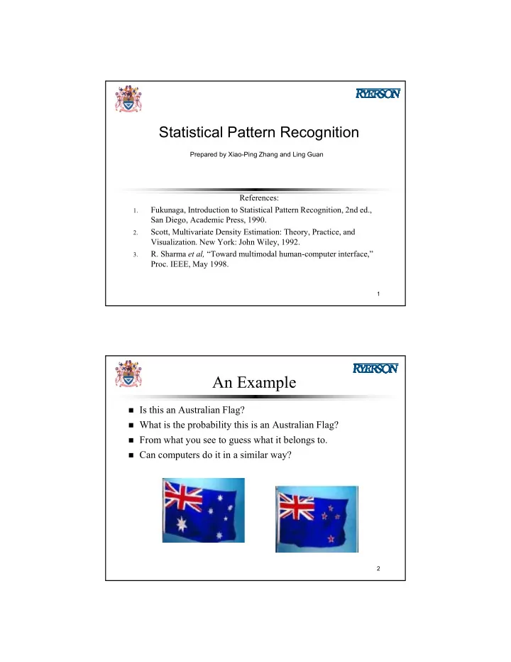
An Example
Is this an Australian Flag? What is the probability this is an Australian Flag? From what you see to guess what it belongs to. Can computers do it in a similar way?