An analysis of faster convergence in certain finance applications - PowerPoint PPT Presentation
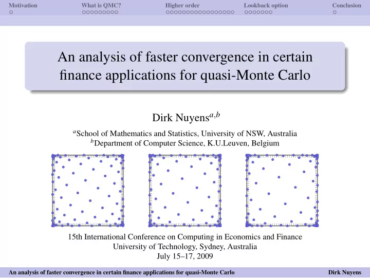
Motivation What is QMC? Higher order Lookback option Conclusion An analysis of faster convergence in certain finance applications for quasi-Monte Carlo Dirk Nuyens a , b a School of Mathematics and Statistics, University of NSW, Australia b
Motivation What is QMC? Higher order Lookback option Conclusion An analysis of faster convergence in certain finance applications for quasi-Monte Carlo Dirk Nuyens a , b a School of Mathematics and Statistics, University of NSW, Australia b Department of Computer Science, K.U.Leuven, Belgium 15th International Conference on Computing in Economics and Finance University of Technology, Sydney, Australia July 15–17, 2009 An analysis of faster convergence in certain finance applications for quasi-Monte Carlo Dirk Nuyens
Motivation What is QMC? Higher order Lookback option Conclusion New things have happened Motivation A paper by Boyle, Lai and Tan (2005) discusses the usage of lattice rules (a quasi-Monte Carlo technique) for derivative pricing. Shows very impressive results using quasi-Monte Carlo methods. (Their paper is a good introduction to QMC for finance.) Lattice rules perform dramatically better than Monte Carlo and even Sobol’ (a favorite quasi-Monte Carlo method in finance). But: Nevertheless: lattice rules are not the magic bullet. Fact: the periodization used is a very delicate process in practice. Since then, there is new technology and theory: Lattice sequences (instead of fixed lattice rules); Higher order digital nets . This talk tries to address these new developments. An analysis of faster convergence in certain finance applications for quasi-Monte Carlo Dirk Nuyens
Motivation What is QMC? Higher order Lookback option Conclusion The problem What is QMC? The underlying numerical problem we are solving is approximating � I ( f ) := [ 0 , 1 ] s f ( x ) d x , by an equal-weight quadrature/cubature rule N − 1 k = 0 ) := 1 � Q ( f , { x k } N − 1 f ( x k ) . N k = 0 If the points x k ( ≡ samples ≡ paths) are taken (pseudo) randomly, then this the Monte Carlo method; 1 deterministically, then this is the Quasi-Monte Carlo method, 2 using low-discrepancy points. E.g., using Sobol’ & Niederreiter sequences or lattice sequences. An analysis of faster convergence in certain finance applications for quasi-Monte Carlo Dirk Nuyens
Motivation What is QMC? Higher order Lookback option Conclusion The problem Derivative pricing. . . Lets assume a stock to adhere to S ( t ) ∼ S ( t 0 ) e ( µ − σ 2 / 2 ) t + σ W ( t ) , with W ( t ) ∼ BM ( 0 , 1 ) , and thus W ( t ) ∼ N ( 0 , t ) , then for a discretization on 0 = t 0 < t 1 < . . . < t n = T we have W := ( W ( t 1 ) , W ( t 2 ) , . . . , W ( t n )) ⊤ ∼ N n ( 0 , C ) , with C i , j = min ( t i , t j ) . An analysis of faster convergence in certain finance applications for quasi-Monte Carlo Dirk Nuyens
Motivation What is QMC? Higher order Lookback option Conclusion The problem . . . as a multi-dimensional integral Since the price of a derivative contract is defined as the expected payoff; this expectation can be written as an integral over all possible underlier paths. Since W ∼ N n ( 0 , C ) , the payoff is given by 2 w ⊤ C − 1 w ) R n g ( w ) exp ( − 1 � E ( payoff ) = d w � ( 2 π ) n det ( C ) R n g ( A z ) exp ( − 1 2 z ⊤ z ) � = d z � ( 2 π ) n � [ 0 , 1 ] n g ( A Φ − 1 ( x )) d x , = for some factorization C = AA ⊤ . An analysis of faster convergence in certain finance applications for quasi-Monte Carlo Dirk Nuyens
Motivation What is QMC? Higher order Lookback option Conclusion Low-discrepancy point sets What sample points to use? Figure: Three point sets with each 64 samples in the unit square. The product left-rectangle rule. → Classical product rule 1 Note: grids don’t work for high dimensions since, e.g., taking the minimum 2 points per dimensions in 100 dimensions requires a total of 2 100 = 1267650600228229401496703205376 points.. . ≈ 10 30 , a quintillion → Monte Carlo Pseudo-random numbers. 2 → Quasi-Monte Carlo Low-discrepancy points . 3 An analysis of faster convergence in certain finance applications for quasi-Monte Carlo Dirk Nuyens
Motivation What is QMC? Higher order Lookback option Conclusion Low-discrepancy point sets What sample points to use? Figure: Three point sets with each 64 samples in the unit square. The product left-rectangle rule. → Classical product rule 1 → Monte Carlo Pseudo-random numbers. 2 (Fig: mt19937, the Mersenne Twister, with default initial state.) → Quasi-Monte Carlo Low-discrepancy points . 3 (Fig: A good lattice sequence in base 3.) An analysis of faster convergence in certain finance applications for quasi-Monte Carlo Dirk Nuyens
Motivation What is QMC? Higher order Lookback option Conclusion Low-discrepancy point sets Lattice rules and sequences An N -point lattice rule with generating vector z ∈ Z s : x k = k z N mod 1 , for k = 0 , 1 , . . . , N − 1 . A lattice sequence generates points x k = ϕ b ( k ) z mod 1 , for k = 0 , 1 , . . . , with ϕ b a “good permutation”. E.g. radical inverse in base b . Figure: A lattice sequence in base 3 with maximal 729 = 3 6 points and z = [ 1 , 140 , . . . ] stopped at 81, 100, 600, 700 and 729 points. An analysis of faster convergence in certain finance applications for quasi-Monte Carlo Dirk Nuyens
Motivation What is QMC? Higher order Lookback option Conclusion Low-discrepancy point sets Digital sequences (e.g., Sobol’ and Niederreiter sequence) A digital sequence in base b (for efficiency, think b = 2) generates points { x k } b m − 1 k = 0 by taking for the j -th dimension x k , j = C j � � k , i.e., · · · x k , j , 1 C j , 1 , 1 C j , 1 , m k 0 . . . . ... . = . . . over F b , . . . . x k , j , m C j , m , 1 · · · C j , m , m k m − 1 where the x k , j , i , for i = 1 , . . . , m , and k i , for i = 0 , . . . , m − 1, are the base b digits of x j and k , m m − 1 x k , j , i b − i ∈ [ 0 , 1 ) , k i b i ∈ Z b m . � � x k , j = k = i = 1 i = 0 (In reality this can be a little bit more complicated.) An analysis of faster convergence in certain finance applications for quasi-Monte Carlo Dirk Nuyens
Motivation What is QMC? Higher order Lookback option Conclusion Low-discrepancy point sets Lattice sequences Note: “lattice” here has *nothing* to do with binomial pricing. A lattice sequence in base b (again, think b = 2) generates points { x k } b m − 1 k = 0 by setting x k = ϕ b ( k ) z mod 1 , where typically ϕ b is the radical inverse in base b (or its Gray code variant). E.g., the radical inverse φ b just reverses the digits: m − 1 m − 1 � � k i b − m − 1 , k i b i . φ b ( k ) := k = given i = 0 i = 0 Typically for a digital sequence C 1 = I , the identity matrix, and for a lattice sequence z 1 = 1. Then the first dimensions coincide. (And form the van der Corput sequence.) An analysis of faster convergence in certain finance applications for quasi-Monte Carlo Dirk Nuyens
Motivation What is QMC? Higher order Lookback option Conclusion Digital sequences versus lattice sequences Digital versus lattice sequences: Practical differences For a digital sequence one needs good generating matrices C 1 , C 2 , . . . , C s ∈ F m × m ; b preferably base 2, then each of the columns of the matrices can be represented by an integer and adding up columns is done by xor ’ing; preferably the k ’s are taken in Gray code ordering such that only one column has to be xor ’d to the previous result when generating sequence elements. For a lattice sequence one needs a good generating vector z ∈ Z s b m ; multiplication modulo 1 is no problem at all; preferably base 2, then radical inverse can be done by bit masks in O ( log 2 ( m )) ; or Gray code variant by 2 assembly instructions. An analysis of faster convergence in certain finance applications for quasi-Monte Carlo Dirk Nuyens
Motivation What is QMC? Higher order Lookback option Conclusion Some examples of usage Pricing of an Asian option 10 1 10 0 10 − 1 10 − 2 std. err. 10 − 3 asian-64-random asian-64-sobol asian-64-lattice 10 − 4 asian-64-sobol-BB asian-64-lattice-BB 10 − 5 asian-64-sobol-PCA asian-64-lattice-PCA 10 − 6 10 0 10 1 10 2 10 3 10 4 10 5 10 6 n Figure: 64 dimensions, 10 random shifts An analysis of faster convergence in certain finance applications for quasi-Monte Carlo Dirk Nuyens
Motivation What is QMC? Higher order Lookback option Conclusion Some examples of usage Pricing of an Asian option 10 1 10 0 Monte Carlo 10 − 1 10 − 2 std. err. std. err. 10 − 3 Order-2 lattice 10 − 4 10 − 5 10 − 6 10 0 10 1 10 2 10 3 10 4 10 5 10 6 n n Figure: 100 dimensions, 10 random shifts An analysis of faster convergence in certain finance applications for quasi-Monte Carlo Dirk Nuyens
Motivation What is QMC? Higher order Lookback option Conclusion The need for speed A reprise on the multivariate integration We are interested in approximating � I ( f ) := [ 0 , 1 ] s f ( x ) d x by some quadrature / cubature rule of the form N − 1 � Q N ( f ; { x k } k , { w k } k ) := w k f ( x k ) . k = 0 For moderate to high dimensions: equal weights w k = N − 1 are nice, with random points ( Monte Carlo , error O ( N − 1 / 2 ) ); or low-discrepancy points ( quasi-Monte Carlo , error ∼ O ( N − 1 ) ). Here: not so interested in high dimensions and wish error ∼ O ( N − α ) . An analysis of faster convergence in certain finance applications for quasi-Monte Carlo Dirk Nuyens
Recommend
More recommend
Explore More Topics
Stay informed with curated content and fresh updates.

