Amortized Analysis Amortization is an analysis technique that can - - PDF document

Meeting 8 September 22, 2005

Amortized Analysis

Amortization is an analysis technique that can influence the design of algorithms in a profound way. Later in this course, we will encounter data structures that owe their very existence to the insight gained in performance due to amortized analysis. Binary counting. We illustrate the idea of amortization by analyzing the cost of counting in binary. Think of an integer as a linear array of bits, n =

i≥0 A[i] · 2i. The

following loop keeps incrementing the integer stored in A. loop i = 0; while A[i] = 1 do A[i] = 0; i++ endwhile ; A[i] = 1. forever . We define the cost of counting as the total number of bit changes that are needed to increment the number one by

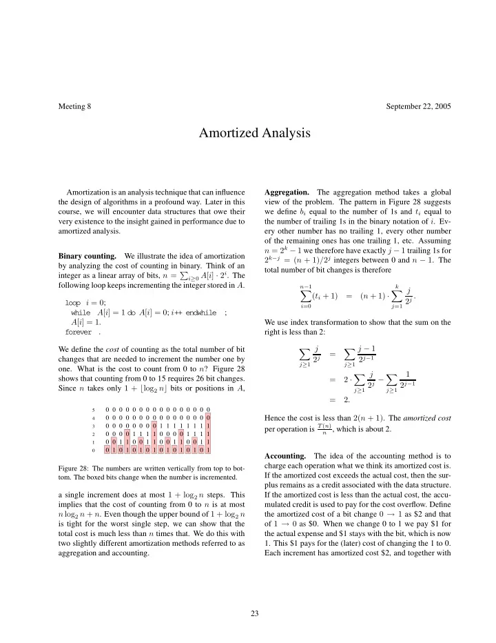
• ne. What is the cost to count from 0 to n? Figure 28

shows that counting from 0 to 15 requires 26 bit changes. Since n takes only 1 + ⌊log2 n⌋ bits or positions in A,

1 1 1 1 1 1 1 1 1 1 1 1 1 1 1 1 0 1 1 1 1 1 1 1 1 1 1 1 1 1 1 1 1

5 4 3 2 1

Figure 28: The numbers are written vertically from top to bot-

• tom. The boxed bits change when the number is incremented.

a single increment does at most 1 + log2 n steps. This implies that the cost of counting from 0 to n is at most n log2 n + n. Even though the upper bound of 1 + log2 n is tight for the worst single step, we can show that the total cost is much less than n times that. We do this with two slightly different amortization methods referred to as aggregation and accounting. Aggregation. The aggregation method takes a global view of the problem. The pattern in Figure 28 suggests we define bi equal to the number of 1s and ti equal to the number of trailing 1s in the binary notation of i. Ev- ery other number has no trailing 1, every other number

• f the remaining ones has one trailing 1, etc. Assuming

n = 2k − 1 we therefore have exactly j − 1 trailing 1s for 2k−j = (n + 1)/2j integers between 0 and n − 1. The total number of bit changes is therefore

n−1

• i=0

(ti + 1) = (n + 1) ·

k

• j=1

j 2j . We use index transformation to show that the sum on the right is less than 2:

• j≥1

j 2j =

• j≥1

j − 1 2j−1 = 2 ·

• j≥1

j 2j −

• j≥1

1 2j−1 = 2. Hence the cost is less than 2(n + 1). The amortized cost per operation is T (n)

n , which is about 2.

Accounting. The idea of the accounting method is to charge each operation what we think its amortized cost is. If the amortized cost exceeds the actual cost, then the sur- plus remains as a credit associated with the data structure. If the amortized cost is less than the actual cost, the accu- mulated credit is used to pay for the cost overflow. Define the amortized cost of a bit change 0 → 1 as $2 and that

• f 1 → 0 as $0. When we change 0 to 1 we pay $1 for

the actual expense and $1 stays with the bit, which is now

• 1. This $1 pays for the (later) cost of changing the 1 to 0.

Each increment has amortized cost $2, and together with 23

the money in the system, this is enough to pay for all the bit changes. The cost is therefore at most 2n. We see how a little trick, like making the 0 → 1 changes pay for the 1 → 0 changes, leads to a very simple analysis that is even more accurate than the one obtained by aggre- gation. Potential functions. We can further formalize the amor- tized analysis by using a potential function. The idea is similar to accounting, except there is no explicit credit saved anywhere. The accumulated credit is an expres- sion of the well-being or potential of the data structure. Let ci be the actual cost of the i-th operation and Di the data structure after the i-th operation. Let Φi = Φ(Di) be the potential of Di, which is some numerical value depending on the concrete application. Then we define ai = ci + Φi − Φi−1 as the amortized cost of the i-th

• peration. The sum of amortized costs of n operations is

n

• i=1

ai =

n

• i=1

(ci + Φi − Φi−1) =

n

• i=1

ci + Φn − Φ0. We aim at choosing the potential such that Φ0 = 0 and Φn ≥ 0 because then we get ai ≥ ci. In words, the sum of amortized costs covers the sum of actual costs. To apply the method to binary counting we define the po- tential equal to the number of 1s in the binary notation, Φi = bi. It follows that Φi − Φi−1 = bi − bi−1 = (bi−1 − ti−1 + 1) − bi−1 = 1 − ti−1. The actual cost of the i-th operation is ci = 1 + ti−1, and the amortized cost is ai = ci + Φi − Φi−1 = 2. We have Φ0 = 0 and Φn ≥ 0 as desired, and therefore ci ≤ ai = 2n, which is consistent with the analysis

• f binary counting with the aggregation and the account-

ing methods. 2-3-4 trees. As a more complicated application of amor- tization we consider 2-3-4 trees and the cost of restructur- ing them under insertions and deletions. We have seen 2-3-4 trees earlier when we talked about red-black trees. A set of keys is stored in sorted order the internal nodes of a 2-3-4 tree, which is characterized by the following rules: (1) each internal node has 2 ≤ d ≤ 4 children and stores d − 1 keys; (2) all leaves have the same depth. As for binary trees, being sorted means that the inorder sequence of the keys is sorted. The only meaningful def- inition of the inorder sequence is the inorder sequence of the first subtree followed by the first key stored in the root followed by the inorder sequence of the second subtree followed by the second key, etc. To insert a new key we attach a new leaf and add the key to the parent ν of that leaf. All is fine unless ν overflows because it now has five children. If it does we repair the violation of Rule (1) by climbing the tree one node at a

• time. We call an internal node non-saturated if it has fewer

than four children. Case

• 1. ν has five children and a non-saturated sibling

to its left or right. Move one child from ν to that sibling, as in Figure 29.

$1 $0 $6 $3 Figure 29: The overflowing node gives one child to a non- saturated sibling.

Case

• 2. ν has five children and no non-saturated sib-
• ling. Split ν into two nodes and recurse for the parent
• f ν, as in Figure 30. If ν has no parent then create a

new root whose only children are the two nodes ob- tained from ν.

$0 $6 $3 $6 $1 Figure 30: The overflowing node is split into two and the parent is treated recursively.

Deleting a key is done is a similar fashion, although there we have to battle with nodes ν that have too few children rather than too many. Let ν have only one child. We repair Rule (1) by adopting a child from a sibling or by merging 24

ν with a sibling. In the latter case the parent of ν looses a child and needs to be visited recursively. The two opera- tions are illustrated in Figures 31 and 32.

$4 $3 $1 $0 Figure 31: The underflowing node receives one child from a sib- ling. $1 $4 $0 $1 $0 Figure 32: The underflowing node is merged with a sibling and the parent is treated recursively.

Amortized analysis. The worst case for inserting a new key occurs when all internal nodes are saturated. The in- sertion then triggers logarithmically many splits. Symmet- rically, the worst case for a deletion occurs when all inter- nal nodes have only two children. The deletion then trig- gers logarithmically many mergers. Nevertheless we can show that in the amortized sense there are at most a con- stant number of split and merge operations per insertion and deletion. We use the accounting method and store money in the internal nodes. The best internal nodes have three children because then they are flexible in both directions. They require no money, but all other nodes are given a posi- tive amount to pay for future expenses caused by split and merge operations. Specifically, we store $4, $1, $0, $3, $6 in each internal node with 1, 2, 3, 4, 5 children. As il- lustrated in Figures 29 and 31, an adoption moves money

• nly from ν to its sibling. The operation keeps the total

amount the same or decreases it, which is even better. As shown in Figure 30, a split frees up $5 from ν and spends at most $3 on the parent. The extra $2 pay for the split

• peration. Similarly, a merger frees $5 from the two af-

fected nodes and spends at most $3 on the parent. This is illustrated in Figure 32. An insertion makes an initial investment of at most $3 to pay for creating a new leaf. Similarly, a deletion makes an initial investment of at most $3 for destroying a leaf. This implies that for n insertions and deletions we get at most 3n

2 split and merge opera-

• tions. In other words, the amortized number of split and

merge operations is at most 3

2.

Recall that there is a one-to-one correspondence be- tween 2-3-4 tree and red-black trees. We can thus trans- late the above update procedure and get an algorithm for red-black trees with an amortized constant restructuring cost per insertion and deletion. We already proved that for red-black trees the number of rotations per insertion and deletion is at most a constant. The above argument im- plies that also the number of promotions and demotions is at most a constant, although in the amortized and not in the worst-case sense as for the rotations. 25