A DVANCED A NALYSIS : A MORTIZATION AND R ECURRECNE R ELATIONS - PDF document

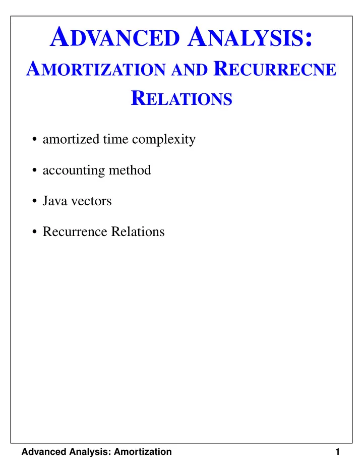
A DVANCED A NALYSIS : A MORTIZATION AND R ECURRECNE R ELATIONS • amortized time complexity • accounting method • Java vectors • Recurrence Relations Advanced Analysis: Amortization 1

Amortized Running Time • Amortized running time considers interactions between operations by studying the total running time of a series of operations. • Example: a Clearable Stack : supports the usual stack methods plus operation clearStack():Empty the stack by removing all all its elements Input: None; Output: None clearStack takes O(n) time in the worst case • Proposition: A series of n operations on an initially empty clearable stack implemented with an array takes overall O(n) time • Justification: - Let M 0 ..., M n-1 be the series of operations and M i 0 ..., M i k -1 be the k-th clearStack operations in the series - We define i -1 = -1 - The run time of operation M i j is O(i j -i j -1 ) since at most i j - i j-1 elements can be on the stack Advanced Analysis: Amortization 2

Amortized Running Time (cont) - Thus the running time of all the clearStack operations is – 1 k   ( ) ∑ – O i j i j   – 1 j = 0 which is a telescoping sum. - So the run time is O(n) • Definition: the amortized running time of an operation within a series of operations is the worst- case running time of the entire series of operations divided by the number of operations. Advanced Analysis: Amortization 3

Accounting Method • The accounting method performs an amoritzation analysis with a system of credits and debits • Let’s view the computer as vending machine that requires one cyber-dollar for a constant amount of computing time. • An operation consists of a series of constant-time primitive operations that cost one cyber-dollar each. • We will overcharge an operation that executes few primitives and use the profit to pay for operations that execute many primitives. • We will need to set up a scheme for charging operations. This is known as the amoritization scheme. Advanced Analysis: Amortization 4

Amortization Scheme Example for a ClearableStack • Assume one cyber-dollar is enough to pay for the push, pop, top, size, or isEmpty and for the time spent by the clearStack to dereference one element. • We will charge 2 cyber-dollars though. • So we undercharge clearStack but overcharge the other operations. When a clearStack operation is executed, the cyber-dollars stored in the stack are used to pay for derefencing the items. $ $ $ $ $ $ $ $ $ $ 0 1 2 3 4 5 6 7 8 9 10 11 12 13 14 15 Advanced Analysis: Amortization 5

Java Vectors • The java.util.vector class provides a convenient expandable data type in Java. • A vector is a wrapper around an array that holds a variable called capacityIncrement . When the user inserts the n +1 st element into a vector of size n, the size of the array is increased by capacityIncrement if it is positive, or doubled if capacityIncrement is 0. • Consider the case of capacityIncrement =0: - Copying an array into a larger array takes O( n ) time, but this only happens for log( n ) insertions. - Each insertion has O(1) amortized running time 1 2 3 4 5 6 7 8 9 10 11 12 13 14 15 16 Advanced Analysis: Amortization 6

Java Vectors (contd.) • Justification: The array doubles in size with the insertion of every 2 i th element (1 st , 2 nd , 4 th , etc.) Worst case: we insert exactly n = 2 i elements, so the last operation involves copying the entire array over again. We have n insertions, and n elements copied in the last insertion. We also have i-1 previous expansions of the array, which perform the following number of element-copy operations: – 1 i 2 k 2 i ∑ = – 1 = – 1 n = 1 k • The overall time complexity is proportional to 3 n -1, which is O( n ) • But what if the capacityIncrement is, say, 3? Do we still have the same amortization? - No! Copying an array into a larger array is O( n ), but this happens once every n / capacityIncrement insertions. - Each insertion is amortized to O( n ) Advanced Analysis: Amortization 7

Java Vectors (contd.) • Justification:(c = capacityIncrement ) Let us assume that the original vector size is 0. The vector increases in size by the insertion of every (ic) th element (1 st , c th , 2*c th , etc.) Worst case: we insert exactly n = ic elements, so the last operation involves copying the entire array. We have n insertions, and n elements copied on the last insertion. We also have i-1 other array copies, for a total of: – 1 – 1 i i ( ) – 1 ci i ∑ ∑ - - - - - - - - - - - - - - - - - = = ck c k 2 = 0 = 0 k k previous element copies. • The overall time complexity is proportional to n ( n -1/(2c)), which is O( n 2 ) Advanced Analysis: Amortization 8

Recurrence Relations Advanced Analysis: Amortization 9

The Pizza Slicing Problem How many pieces of pizza can you get with N straight cuts ? 1 cut 2 cuts 3 cuts 2 slices 4 slices 6 slices ... But ... who said you should cut N cuts through the center every time? 2N slices Advanced Analysis: Amortization 10

A Better Slicing Method ... When cutting, intersect all previous cuts and avoid previous intersection points! 4 cuts 11 slices!! 5 cuts 16 slices!! Advanced Analysis: Amortization 11

So ... How Many Pieces? 3 cuts 4 cuts 5 cuts 7 slices 11 slices 16 slices The N-th cut creates N new pieces. Hence, the total number of pieces given by N cuts, denoted P(N), is given by the following two rules: • P(1) = 2 • P(N) = P(N-1) + N Recursive definition of P(N)! Advanced Analysis: Amortization 12

Recurrence Relations • The pizza-cutting problem is an example of recurrence relation , where a function f ( N ) is recursively defined. ( ) f 1 = 2 (Base Case) ( ) ( ) for N ≥ 2 = – 1 + f N f N N (Recursive Case) • The standard method for solving recurrence relations, called“unfolding”, makes repeated substitutions applying the recursive rule until the base case is reached. ( ) ( ) = – 1 + f N f N N ( ) ( ) ( ) = – 2 + – 1 + f N f N N N ( ) ( ) ( ) ( ) = – 3 + – 2 + – 1 + f N f N N N N ... ( ) ( ) ( ) … ( ) = – i + – i + 1 + + – 1 + f N f N N N N The base case is reached when i = N − 1 ( ) … ( ) ( ) = 2 + 2 + 3 + + – 2 + – 1 + f N N N N ( ) + 1 N N O N 2 ( ) ( ) - - - - - - - - - - - - - - - - - - = + 1 = f N 2 Advanced Analysis: Amortization 13

Towers of Hanoi A C B Goal: transfer all N disks from peg A to peg C Rules: • move one disk at a time • never place larger disk above smaller one Recursive solution: • transfer N − 1 disks from A to B • move largest disk from A to C • transfer N − 1 disks from B to C Total number of moves: • T( N ) = 2 T( N − 1) + 1 Advanced Analysis: Amortization 14

Solution of the Recurrence for Towers of Hanoi Recurrence relation: • T( N ) = 2 T( N − 1) + 1 • T(1) = 1 Solution by unfolding: T( N ) = 2 ( 2 T( N − 2) + 1 ) + 1 = = 4 Τ( N − 2) + 2 + 1 = = 4 ( 2 Τ( N − 3) + 1 ) + 2 + 1 = = 8 Τ( N − 3) + 4 + 2 + 1 = ... = 2 i T( N − i) + 2 i − 1 + 2 i −2 + ... + 2 1 + 2 0 the expansion stops when i = N − 1 T( N ) = 2 N − 1 + 2 N − 2 + 2 N −3 + ... + 2 1 + 2 0 This is a geometric sum , so that we have: T( N ) = 2 N − 1 = Ο (2 N ) Advanced Analysis: Amortization 15

Another Recurrence   2 T N ( ) ≥ = - - - - + T N N for 2   N 2 ( ) T 1 = 1     2 2 T N N T ( N ) = - - - - + - - - - + N     4 2   4 T N = - - - - + 2 N   4     4 2 T N N = - - - - + - - - - + 2 N     8 4   8 T N = - - - - + 3 N   T (1) = 1 8 … =   2 iT N   - - - - + iN   2 i The expansion stops for i = log N, so that … T( N ) = N + N log N Advanced Analysis: Amortization 16

Solving Recurrences by “Guess and Prove”   2 T N ( ) ≥ = - - - - + T N N for 2   N 2 ( ) T 1 = 1 Step 1: Take a wild guess that ( ) = + log T N N N N Step 2: Prove it by induction: Basis ( ) T 1 = 1 + log 1 = 1 Inductive Step     2 T N N 2 N N ( ) = - - - - + = - - - - + - - - - log - - - - + T N N N     2 2 2 2 ( ) ( ) = + log – 1 + = + log T N N N N N N N N Advanced Analysis: Amortization 17

A More Difficult Example ( ) ( ) ( ) = 2 T + 1 T 2 = 0 T N N 2 T N 1 2 / ( ) + 1 2 2 T N 1 4 / ( ( ) ) + 1 + 1 4 T N 1 4 / ( ) + 1 + 2 8 T N 1 8 / ( ) + 1 + 2 + 4 … 1   - - - - 2 i   20 21 – 1 2 iT N 2 i … + + + +     1 - - - - 2 i The expansion stops for = 2 N i.e., i = loglog N 20 21 log log – 1 N ( ) … = + + + 2 = log – T N N Advanced Analysis: Amortization 18

Proofs by Induction We want to show that property P is true for all integers n ≥ n 0 Basis: prove that P is true for n 0 . Inductive Step: prove that if P is true for all k such that n 0 ≤ k ≤ n − 1 then P is also true for n Advanced Analysis: Amortization 19