
SLIDE 1
Jan S Hesthaven EPFL-SB-MATH-MCSS Jan.Hesthaven@epfl.ch
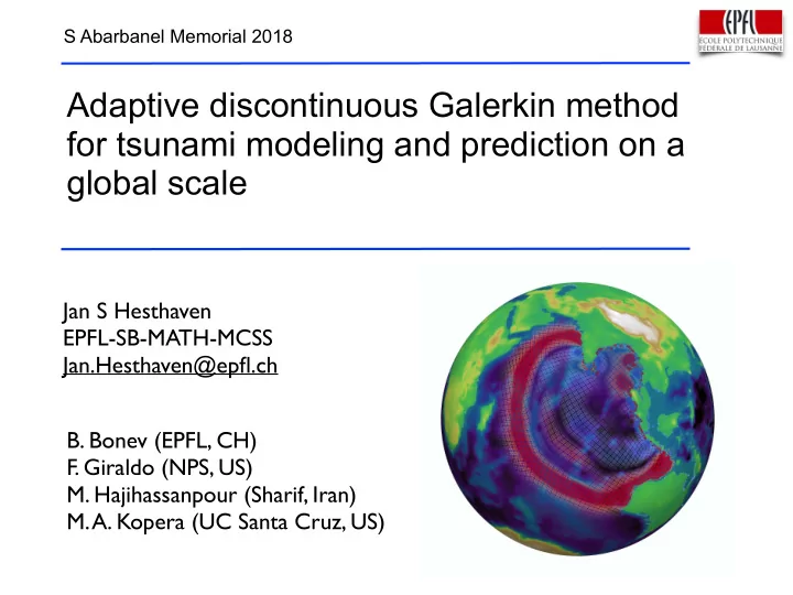
Adaptive discontinuous Galerkin method for tsunami modeling and prediction on a global scale
S Abarbanel Memorial 2018- B. Bonev (EPFL, CH)
- F. Giraldo (NPS, US)
- M. Hajihassanpour (Sharif, Iran)
- M. A. Kopera (UC Santa Cruz, US)