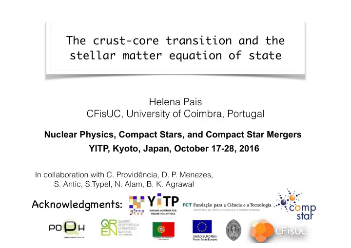
Acknowledgments: One of the most dense objects in Universe: - - PowerPoint PPT Presentation

The crust-core transition and the stellar matter equation of state

Helena Pais CFisUC, University of Coimbra, Portugal

Nuclear Physics, Compact Stars, and Compact Star Mergers YITP, Kyoto, Japan, October 17-28, 2016

In collaboration with C. Providência, D. P. Menezes,

• S. Antic, S.Typel, N. Alam, B. K. Agrawal

Acknowledgments:

Neutron stars

• One of the most dense objects in Universe:

R~10km and M~1.5 1.Outer crust 2.Inner crust 3.Core

M

N . C h a m e l a n d P . H a e n s e l . L i v . R e v . R e l . 1 1 , 1 , 2 8

• The choice of inner crust EoS and the matching to the core EoS

can be critical :

• Divided in 3 main layers:

Variations have been found of 0.5km for a M=1.4 star!

M

Crust-core transition important:

• plays crucial role in fraction of I in crust of star:

Pt

Icrust ∼ 16π 3 R6

t Pt

Rs which also depends on crust thickness, Rt

Describing neutron stars

1.EoS: for a system at given and 2.Compute TOV equations 3.Get star M(R) relation ρ T P(E) Prescription: Problem: Which EoS to choose?

• Phenomenological models (parameters are fitted to nuclei

properties): RMF, Skyrme…

• Microscopic models (starts from n-body nucleon

interaction): (D)BHF, APR… Solution: Need Constrains!! Many EoS models in literature:

P . B . D e m

• r

e s t e t a l , N a t u r e 4 6 7 , 1 8 1 , 2 1

1 10 100 1 2 3 4 P (MeV fm-3) /0 T=0, yp=0.5 Experiments flow exp. KaoS exp.

EoS Constrains

• Experiments
• P. Danielewicz et al,

Science 298, 1592, 2002

• W. G. Lynch et al,

PPNP 62, 427 2009

• Microscopic calculations
• S. Gandolfi et al,

PRC 85, 032801, 2012

• K. Hebeler et al,
• Astrophys. J. 773,11, 2013
• Observations
• J. M. Lattimer and M. Prakash,

arXiv: 1012.3208 [astro-ph.SR] 2010 0.1 0.2 0.4 0.6 1 2 3 0.02 0.04 0.06 0.08 0.1 0.12 0.14 0.16 P (MeV fm-3) (fm-3) T=0, neutron matter Microscopic calculations Chiral EFT Monte Carlo

• J. M. Lattimer and A. W Steiner,

EPJA 50, 40, 2014

Choosing the EoS(s)

We need unified EoS, but if we don’t have it..

!

Choose 1 EoS for each NS layer:

!

• Outer crust EoS (BPS or HP or RHS)
• Inner crust EoS (1)
• Core EoS

arXiv:1604.01944 [astro-ph.SR] 2016

M(R) not affected pasta phases ?, unified core EoS ? homogeneous matter

• Match OC EoS at the neutron drip with IC EoS
• Match IC EoS at crust-core transition (2) with Core EoS

and then We are going to focus on (1) and (2) to obtain the transition densities and pressures!

The pasta phases

• Competition between Coulomb and nuclear forces leads to

frustrated system

• Geometrical structures, the pasta phases, evolve with density

until they melt crust-core transition

• Criterium: pasta free energy must be lower than the

correspondent hm state

• G. Watanabe et al, PRL 103, 121101, 2009
• C. J. Horowitz et al, PRC 70, 065806, 2004

QMD calculations:

Pasta phases - calculation (I)

• Thomas-Fermi (TF) approximation:
• Nonuniform npe matter system described inside Wigner-Seitz cell:!

! Sphere, cilinder or slab in 3D (spherical symmetry), 2D (axial symmetry ! ! ! around z axis) and 1D (reflexion symmetry).!

• Matter is assumed locally homogeneous and, at each point, its density is

determined by the corresponding local Fermi momenta. !

• Fields are assumed to vary slowly so that baryons can be treated as

moving in locally constant fields at each point. !

• Surface effects are treated self-consistently. !
• Quantities such as the energy and entropy densities are averaged over the
• cells. The free energy density and pressure are calculated from these

two thermodynamical functions.

Pasta phases - calculation (II)

• Coexistence Phase (CP) approximation:
• Separated regions of higher and lower density: pasta phases, and a

background nucleon gas.!

• Gibbs equilibrium conditions: for : !

!

• Finite size effects are taken into account by a surface and a Coulomb

terms in the energy density, after the coexisting phases are achieved.!

• Total and total of the system:


!

!

µI

p = µII p

µI

n = µII n

P I = P II T = T I = T II F = fFI + (1 − f)FII + Fe + ✏surf + ✏coul F ρp ρp = ρe = ypρ = fρI

p + (1 − f)ρII p

check PRC 91, 055801 2015

Pasta phases - calculation (III)

• Compressible Liquid Drop (CLD) approximation:

The total free energy density is minimized, including the surface and Coulomb terms. The equilibrium conditions become: µI

n = µII n ,

P I = P II − ✏surf ⇣ 1 2↵ + 1 2 @ @f − ⇢II

p

f(1 − f)(⇢I

p − ⇢II p )

⌘ µI

p = µII p −

✏surf f(1 − f)(⇢I

p − ⇢II p ),

check PRC 91, 055801 2015

Non-linear Walecka Model

nucleons electrons mesons em non-linear mixing couplings

Li = ¯ ψi [γµiDµ − M ∗] ψi

Le = ¯ ψe [γµ (i∂µ + eAµ) − me] ψe

Lσ = 1 2 ✓ ∂µφ∂µφ − m2

sφ2 − 1

3κφ3 − 1 12λφ4 ◆

Lω = −1 4ΩµνΩµν + 1 2m2

vVµV µ + 1

4!ξg4

v(VµV µ)2

Lρ = −1 4Bµν · Bµν + 1 2m2

ρbµ · bµ

Lγ = −1 4FµνF µν

Lσωρ = Λ3σgsg2

vφVµV µ + Λ2σg2 sg2 vφ2VµV µ + Λ1σgsg2 ρφbµ · bµ

+Λσg2

sg2 ρφ2bµ · bµ + Λvg2 vg2 ρbµ · bµVµV µ

L = X

i=p,n

Li + Le + Lγ + Lσ + Lω + Lρ + Lσωρ

mesons: mediation of nuclear force non-linear mixing couplings terms: responsible for density dependence of Esym!

)

−3

(fm

n 0.02 0.04 0.06 0.08

)

−3

(fm

p 0.02 0.04 0.06 0.08

c

• e

x i s t e n c e spinodal binodal

Y =0

• Y =0.4

L

− equil.

• How to calculate transition density?
• Thermodynamical spinodal
• Dynamical spinodal

1) Get the instability region: 2) Intersect EoS with that boundary to get ρt

PRC 82, 055807, 2010 PRC 85, 059904(E), 2012

For -eq. matter and T=0, dyn. spinodal very coincident with TF calculation

β

• r

n

thermodynamical dynamical

p (fm ) −3

(fm )

−3

• 0.02

0.04 0.06 0.08 0.08 0.06 0.04 0.02

courtesy: C. Providência courtesy: C. Providência

Thermodynamical spinodal

• The (free) energy curvature matrix for asymmetric NM is

defined by:

check PRC 74, 024317 2006

C = ⇣ ∂2F ∂ρi∂ρj ⌘

• Stability conditions: Tr(C) > 0, Det(C) > 0
• The spinodal is given by

for which Det(C) = 0 i.e., one of eigenvalues is negative in the region of instability and goes to zero at border: λ− = 1 2 ⇣ Tr(C) − p Tr(C)2 − 4Det(C) ⌘ = 0

(T, ρp, ρn)

The crust-core transition - thermodynamical spinodal approach

D* models: scalar and vector self-energies depend on E: the couplings are adjusted to the

• ptical potential in nuclear

matter.

• Nucl. Phys. A 938, 92 2015

p r e l i m i n a r y ! w i t h S . A n t i c , S . T y p e l a n d C . P r

• v

i d ê n c i a

a) density-dependent models

0.02 0.04 0.06 0.08 0.02 0.04 0.06 0.08 p (fm-3) n (fm-3) T=12 MeV T=6 MeV D1 D2

b) non-linear mixing meson couplings models

e.g. PRC 81, 034323 2010 with N. Alam, B. K. Agrawal and C. Providência p r e l i m i n a r y !

0.02 0.04 0.06 0.08 0.02 0.04 0.06 0.08 p (fm-3) n (fm-3) T=12 MeV T=6 MeV F2 F

Different mixing couplings: different L: L(F)=70 MeV , L(F2)=46 MeV .

Dynamical spinodal

• Dynamical instabilities are given by collective modes that

correspond to small oscillations around equilibrium state.

• These small deviations are described by linearized equations
• f motion.
• Perturbed fields:
• Perturbed distribution function:

Fi = Fi0 + δFi fi = fi0 + δfi

c h e c k P R C 9 4 , 1 5 8 8 2 1 6

• Very good tool to estimate crust-core transition in cold

neutrino-free neutron stars.

check PRC 82, 055807 2010; PRC 85, 059904(E) 2012

Dynamical spinodal (cont)

• We get a set of equations for the fields and particles, whose solutions

form a complete set of eigenmodes, that lead to the following matrix:

• The dynamical spinodal surface is defined by the region in

space, for a given wave vector k and temperature T, limited by the surface

• In the k=0 MeV limit, the thermodynamic spinodal is obtained.

(ρp, ρn) ω = 0.

  1 + F ppLp F pnLp Cpe

A Lp

F npLn 1 + F nnLn Cep

A Le

1 − Cee

A Le

 

  

2PFp 3k δρp ρp 2PFn 3k δρn ρn 2PFe 3k δρe ρe

   = 0

semiclassical approach, that is a good approximation to t-dependent Hartree-Fock eqs at low energies

• The time evolution of the distribution functions is described

by the Vlasov equation:

∂fi ∂t + {fi, hi} = 0, i = p, n, e

The crust-core transition - dynamical spinodal approach

1.The larger L, the smaller the spinodal section. P R C 9 4 , 1 5 8 8 2 1 6 3.Crossing of the ωρ and σρ spinodals, for a given L, occurs close to the crossing

• f the β-eq EoS with

the spinodals ωρ terms

ρt

σρ terms L<80MeV, Pt is larger for ωρ: ! direct implication in I

0.02 0.04 0.06 0.08 0.02 0.04 0.06 0.08 p (fm-3) n (fm-3) T=0 MeV, k=75 MeV L=118, NL3 L=68, 4 4 L=55, 6 6

0.05 0.055 0.06 0.065 0.07 0.075 0.08 0.085 40 50 60 70 80 90 100 110 120 t (fm-3) L (MeV) TM1 NL3 Z271 TM1 NL3 Z271 0.2 0.25 0.3 0.35 0.4 0.45 0.5 0.55 0.6 40 50 60 70 80 90 100 110 120 Pt (MeV.fm-3) L (MeV)

for ωρ or the σρ models about the same. 2.The term ωρ makes the spinodal section larger compared to σρ. but

M(R) relations

Stars with unified inner crust-core EoS (black lines) have larger (smaller) radii than configurations without inner crust (pink lines) for the NL3ωρ (NL3σρ) models.! Effect on Mmax is negligible, not true for the radius!!

a) effect of pasta: b) effect of different inner crust EoS with L close to core EoS:

σρ give slightly larger radii than ωρ models, the differences being larger for M >~ 1.4M⊙. For 1.4M⊙ star, difference is of ∼ 100 m.! the error on the determination of the radius is negligible for all masses! tested for other models (TM1 and Z271): same result!!

0.5 1 1.5 2 2.5 3 13 14 15 16 M (Msun) R (km) bps+pasta+hm bps+hm L=118, NL3 L=55, 6 6

0.5 1 1.5 2 2.5 3 13 14 15 16 M (Msun) R (km) bps+pasta+hm bps+pasta(FSU)+hm PSR J0348+0432 PSR J1614-2230

exceptions: NL3σρ6, difference of ~50 m (∼ 40 m) for a 1M⊙ ( 1.4M⊙) star; NL3ωρ6, ∼ 20 m for a 1M⊙ star We get the transition density from a dyn. spin. calculation.

• 10
• 5

5 10 0.04 0.06 0.08 0.1 0.12 0.14 0.16 (PNM-Pmicro)/ (fm-3) (b) Monte Carlo

• 10
• 5

5 10 0.04 0.06 0.08 0.1 0.12 0.14 0.16 (PNM-Pmicro)/ (fm-3) (a) T=0, neutron matter Chiral EFT NL3 6 6 TM1 6 6 Z271 8 5 6 1 10 100 1 2 3 4 P (MeV fm-3) /0 T=0, yp=0.5 flow exp. KaoS exp. NL3 TM1 Z271 Z271,cut

0.5 1 1.5 2 2.5 3 10 11 12 13 14 15 16 M (Msun) R (km) NL3 TM1 Z271* Z271 NL36 6 TM16 6 Z2715 6 5* 6*

If we combine the 3 constrains, we get the following models:

NL3 did not pass exp. constrain Z271*: extra potential dependent on σ meson, that makes M* to stop decreasing above saturation density, as suggested in K. A. Maslov, E. E. Kolomeitsev, and D. N. Voskresensky, Phys. Rev. C 92, 052801 (2015).

For 1.4M⊙ stars, these models predict R=13.6 ± 0.3 km and a crust thickness

• f 1.36 ± 0.06km.

Z271 did not pass obs. constrain exceptions: and but

• ext. Nambu—Jona-Lasinio Model

P R C 9 3 , 6 5 8 5 2 1 6

• Set of models with chiral symmetry included, unlike RMFs
• Since chiral symmetry is satisfied, EoS valid at higher

densities!

short range repulsion short range attraction

density dependence of scalar coupling isospin asymmetric nuclear matter to make restoration of the chiral symmetry less abrupt make the symmetry energy softer

L = ¯ ψ(iγµ∂µ − m)ψ +Gs[( ¯ )2 + ( ¯ i5~ ⌧ )2] −Gv( ¯ ψγµψ)2

−Gsv[( ¯ )2 + ( ¯ i5~ ⌧ )2]( ¯ µ )2

−Gρ ⇥ ( ¯ µ~ ⌧ )2 + ( ¯ 5µ~ ⌧ )2⇤

−Gvρ( ¯ µ )2 ⇥ ( ¯ µ~ ⌧ )2 + ( ¯ 5µ~ ⌧ )2⇤ −Gsρ ⇥ ( ¯ )2 + ( ¯ i5~ ⌧ )2⇤ ⇥ ( ¯ µ~ ⌧ )2 + ( ¯ 5µ~ ⌧ )2⇤

M = m − 2Gsρs + 2Gsvρsρ2 + 2Gsρρsρ2

3

nucleon effective mass

eNJL models

20 40 60 80 100 120 0.1 0.2 0.3 0.4 0.5 Esym (MeV) (fm-3) eNJL1 eNJL11 eNJL12 eNJL2 eNJL21 eNJL3 eNJL31 20 40 60 80 100 0.1 0.2 0.3 0.4 0.5 Esym (MeV) (fm-3) eNJL1m eNJL1m1 eNJL2m eNJL2m1

• In this study, we used eNJLx, eNJLxωρy, and eNJLxσρy type of models
• We also considered models with a current mass: eNJLxm, and eNJLxmσρy.
• To make Esym softer: *ωρ* and *σρ* models, where we fixed the Esym at ρ=0.1 at the

same value of eNJLx (eNJLxm), and we calculated the new Gρ, fixing the Gvρ (Gsρ) constant.

without current mass with current mass

eNJL models-Constrains

1 10 100 1 2 3 4 5 P (MeV fm-3) /0 (a) T=0, yp=0.5 Flow exp. Kaons exp. eNJL1 eNJL2 eNJL3 eNJL1m eNJL2m

0.5 1 1.5 2 2.5 3 3.5 0.04 0.06 0.08 0.1 0.12 0.14 0.16 P (MeV fm-3) (fm-3) T=0, neutron matter Hebeler et al. Gandolfi et al. eNJL1 eNJL11 eNJL2 eNJL21 eNJL3 eNJL31 eNJL2m eNJL2m1

But the models need to fulfil the constrains…

Experiments Microscopic calculations

• nly 2 models passed:

eNJL3σρ1 and eNJL2mσρ1

M(R) relations

0.5 1 1.5 2 2.5 11 12 13 14 15 16 17 18 M (Msun) R (km) eNJL31

psr J0348+0432 psr J1614-2230 BPS+hm BPS+pasta(CP)+hm BPS+pasta(CLD)+hm

1) outer crust: BPS 2) inner crust: pasta from a CP or CLD calculation 3) core: hom. nucleonic matter, same model as inner crust

1) EoS:

0.5 1 1.5 2 2.5 11 12 13 14 15 16 17 18 M (Msun) R (km) BPS+pasta+hm

psr J0348+0432 psr J1614-2230 eNJL31 eNJL2m1

CP or CLD: no difference in M(R)

eNJL3σρ1: eNJL2mσρ1:

2) integrate TOV 3) get M(R)

R(M=1.4M⊙)=13.212 km, with ∆R(M=1.4M⊙)=1.405km. R(M=1.4M⊙)=13.084 km, with ∆R(M=1.4M⊙)=1.408km.

M(R) relations (cont)

Considering hybrid stars:

• quark core described within SU(3) NJL model

0.5 1 1.5 2 2.5 11 12 13 14 15 M (Msun) R (km) (a) psr J0348+0432 psr J1614-2230 eNJL31+NJL1 eNJL31+NJL2 eNJL31+NJL3 eNJL31+NJL4

We are still able to describe stable 2M⊙ stars with a quark core!! The deconfinement phase transition decreases maximum mass though…

• perform a Maxwell construction to get hadronic to quark transition

Summary

• Inclusion of the inner crust EoS has strong effect on

the radius of low and intermediate mass neutron stars!

• Unified EoS are needed!

but…

• Inner crust EoS with similar symmetry energy

properties as the core EoS: effect on radii for stars with M > 1 M⊙ is negligible!

• For RMF models, R(M=1.4M⊙)=13.6±0.3km, with

∆R(M=1.4M⊙)=1.36±0.06km.

• Inner-crust—core unified EoS with chiral symmetry and

pasta allows the description of 2 M⊙ stars, with R(M=1.4M⊙)=13.148±0.064km.

Strong correlations of neutron star radii with the slopes of nuclear matter incompressibility and symmetry energy at saturation

set of 24 Skyrme-type effective forces and 18 RMF models, and 2 microscopic calculations, all describing 2M⊙ neutron stars. Unified EoSs for the inner-crust-core region have been built for all the phenomenological models, both relativistic and non-relativistic.

• accep. PRC (R), arXiv:

1610.06344[nucl-th]

8 10 12 14 16 R (km) 0.5 1 1.5 2 2.5 3 MNS (MO)

0.5 1 1.5 ρc (fm

• 3)

.

PSR J0348+0432 PSR J1614-2230

240 270 300

K0 (MeV)

2000 2500 3000 3500

M0 (MeV)

12 13 14

R1.0 (km)

40 80 120

L0 (MeV)

12 13 14 15

R1.4 (km)

C(R1.0, K0) = 0.655 C(R1.0, M0) = 0.646 C(R1.0, L0) = 0.850 C(R1.4, K0) = 0.704 C(R1.4,M0) = 0.743 C(R1.4, L0) = 0.745

We started by calculating correlation

• f R with K, M and L…

We found strong correlation of the neutron star R with linear combination of M and L, and almost independent

• f the neutron star mass in the range 0.6-1.8M⊙.

300 350 400 450 500

K0+αL0 (MeV)

250 300 350 400

K0+αL0 (MeV)

12 13 14 15

R1.0 ( km)

3000 4000 5000 6000

M0+βL0 (MeV)

11 12 13 14 15

R1.4 (km)

3000 4000 5000

M0+βL0 (MeV)

C(R1.0, K0+αL0) = 0.902 C(R1.4, K0+αL0) = 0.850 C(R1.0, M0+βL0) = 0.945 C(R1.4, M0+βL0) = 0.924 α = 1.564 α = 0.883 β = 17.089 β = 28.370

and then…

0.6 0.8 1 C(RX , b)

K0 L0 K0+αL0

0.6 0.8 1 1.2 1.4 1.6 1.8

MNS (MO)

0.4 0.6 0.8 1 C(RX , b)

M0 L0 M0+βL0

b {

{

b

.

and…. This correlation can be linked to the empirical relation between R and P at a nucleonic density between 1-2 saturation density, and the dependence of P on K, M and L.

Thank you!