A weighted (directed or undirected graph) is a pair ( G , W ) - PowerPoint PPT Presentation

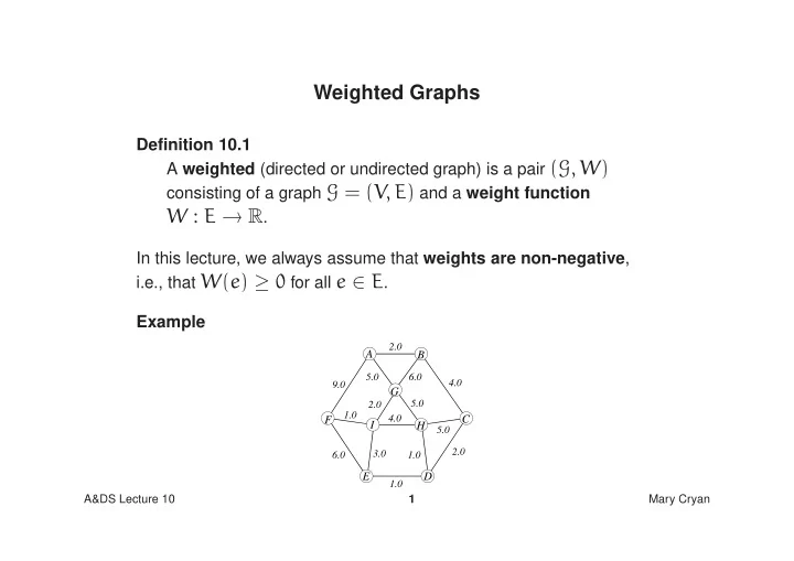
Weighted Graphs Definition 10.1 A weighted (directed or undirected graph) is a pair ( G , W ) consisting of a graph G = ( V, E ) and a weight function W : E → R . In this lecture, we always assume that weights are non-negative , i.e., that W ( e ) ≥ 0 for all e ∈ E . Example 2.0 A B 5.0 6.0 4.0 9.0 G 5.0 2.0 1.0 4.0 C F I H 5.0 2.0 3.0 6.0 1.0 E D 1.0 A&DS Lecture 10 1 Mary Cryan

Representations of Weighted Graphs (as Matrices) 2.0 A B 5.0 6.0 4.0 9.0 G 5.0 2.0 1.0 4.0 C F I H 5.0 2.0 3.0 6.0 1.0 E D 1.0 Adjacency Matrix 0 1 0 2.0 0 0 0 9.0 5.0 0 0 2.0 0 4.0 0 0 0 6.0 0 0 B C B C 0 4.0 0 2.0 0 0 0 5.0 0 B C B C B C 0 0 2.0 0 1.0 0 0 1.0 0 B C B C 0 0 0 1.0 0 6.0 0 0 3.0 B C B C 9.0 0 0 0 6.0 0 0 0 1.0 B C B C 5.0 6.0 0 0 0 0 0 5.0 2.0 B C B C B C 0 0 5.0 1.0 0 0 5.0 0 4.0 @ A 0 0 0 0 3.0 1.0 2.0 4.0 0

Representations of Weighted Graphs (as Adj. lists) 2.0 A B 5.0 6.0 4.0 9.0 G 5.0 2.0 1.0 4.0 F C I H 5.0 2.0 3.0 6.0 1.0 E D 1.0 Adjacency Lists A 2.0 B G 5.0 F 9.0 B G 6.0 C 4.0 A 2.0 C D 2.0 H 5.0 B 4.0 D C 2.0 H 1.0 E 1.0 E 1.0 F D I 3.0 6.0 F A 9.0 I 1.0 E 6.0 G A 5.0 6.0 H 5.0 I 2.0 B H G 5.0 5.0 D 1.0 4.0 C I I F 1.0 G 2.0 H 4.0 E 3.0

Connecting Sites Problem Given a collection of sites and costs of connecting them, find a minimum cost way of connecting all sites. Our formal model • Sites are vertices of a weighted graph , and the weights of the edges represent the cost of connecting their endpoints. • It is reasonable to assume that the graph is undirected and connected . • The cost of a subgraph is the sum of the costs of its edges. • The problem is to find a subgraph of minimum cost that connects all vertices . Compare this to the shortest path problem, where we are only interested in minimum cost connections between pairs of vertices. A&DS Lecture 10 4 Mary Cryan

Spanning Trees G = ( V, E ) undirected connected graph and W weight function. H = ( V H , E H ) with V H ⊆ V and E H ⊆ E subgraph of G . • The weight of H is the number � W ( H ) = W ( e ) . e ∈ E H • H is a spanning subgraph of G if V H = V . Observation 10.2 A connected spanning subgraph of minimum weight is a tree. A&DS Lecture 10 5 Mary Cryan

Minimum Spanning Trees ( G , W ) undirected connected weighted graph Definition 10.3 A minimum spanning tree (MST) of G is a connected spanning subgraph T of G of minimum weight. The minimum spanning tree problem : Undirected connected weighted graph ( G , W ) Input: An MST of G Output: A&DS Lecture 10 6 Mary Cryan

Prim’s Algorithm Idea Grow an MST out of a single vertex by always adding edges of minimum weight. A fringe edge for a subtree T of a graph is an edge with exactly one endpoint in T (so e = ( u, v ) with u ∈ T and v �∈ T ). Algorithm P RIM ( G , W ) 1. T ← one vertex tree with arbitrary vertex of G 2. while there is a fringe edge do add fringe edge of minimum weight to T 3. 4. return T This algorithm uses a Greedy strategy . ** First time we have used the Greedy approach in this course.** A&DS Lecture 10 7 Mary Cryan

Correctness of Prim’s algorithm 1. Throughout the execution of P RIM , T remains a tree. Proof: To show this we need to show that throughout the algorithm, T is (i) always connected and (ii) never contains a cycle . (i) Only edges with an endpoint in T are added to T , so T remains connected. (ii) We never add any edge which has both endpoints in T (we only allow a single endpoint), so the algorithm will never construct a cycle. 2. All vertices will eventually be added to T . Proof: (by contradiction ) This depends on our assumption that the graph G was connected. • Suppose w is a vertex that never gets added to T (as usual, in doing proof by contradiction, our assumption is the opposite of what we want to prove). • Let v = v 0 e 1 v 1 e 2 . . . v n = w be a path from some vertex v inside T to w (we know such a path must exist, because G is connected). Let v i be the first vertex on this path that never got added to T . • After v i − 1 was added to T , e i = ( v i − 1 , v i ) would have become a fringe edge. Also, it would have remained as a fringe edge unless v i was added to T . • So eventually v i would have been added, because Prim’s algorithm only stops if there are no fringe edges. So our assumption was wrong. We must have w in T for every vertex w . 7-1

3. Throughout the execution of P RIM , T is contained in some MST of G . (This will be enough to prove Correctness, because at the end, when all vertices are added, we will have an MST) Proof: (by induction) • Suppose that T is contained in an MST T ′ and that fringe edge e = ( x,y ) is then added to T . We shall prove that T + e is also contained in some MST T ′′ (not necessarily the MST T ′ ). • If e is contained in T ′ , then our proof is easy, we can simply let T ′′ = T ′ . • Otherwise, consider some path P from x to y in T ′ . The path P contains exactly one edge e ′ = ( x ′ ,y ′ ) which is currently (at the time we are adding e = ( x,y ) ) a competing fringe edge for Prim’s algorithm. • Then W ( e ) ≤ W ( e ′ ) (otherwise e ′ would be added instead of e ). • Let T ′′ = T ′ + e − e ′ . • T ′′ is a tree (we add e to make a cycle, then delete e ′ to break it). • T ′′ has the same vertices as T ′ , thus it is a spanning tree. • Moreover, W ( T ′′ ) ≤ W ( T ′ ) , thus T ′′ is also a Minimum Spanning Tree (MST). 7-2

Toward an Implementation Improvement • Instead of fringe edges, we think about adding fringe vertices to the tree. • A fringe vertex is a vertex y not in T that is an endpoint of a fringe edge. • The weight of a fringe vertex y is � � � e = ( x, y ) fringe edge � W ( e ) min • To be able to recover the tree, with each vertex y we store its parent in the tree. We store the fringe vertices in a priority queue . A&DS Lecture 10 8 Mary Cryan

Priority Queues with Decreasing Key A priority queue is an ADT for storing a collection of elements with an associated key - remember Inf 2B . The following methods are supported: • I NSERT ( e, k ) : Insert element e with key k . • G ET -M IN () : Return an element with minimum key; an error occurs if the priority queue is empty. • E XTRACT -M IN () : Return and remove an element with minimum key; an error occurs if the priority queue is empty. • I S -E MPTY () : Return TRUE if the priority queue is empty and FALSE otherwise. To update the keys during the execution of P RIM , we need priority queues supporting the following additional method: • D ECREASE -K EY ( e, k ) : Set the key of e to k and update the priority queue. It is assumed that k is smaller than or equal to the old key of e . A&DS Lecture 10 9 Mary Cryan

Implementation of Prim’s Algorithm Algorithm P RIM ( G , W ) Algorithm R ELAX ( y, z ) ` ´ ( y, z ) 1. Initialise parent array π : 1. w ← W π [ v ] ← NIL for all vertices v 2. if weight [ z ] = ∞ then 2. Initialise weight array: weight [ z ] ← w 3. weight [ v ] ← ∞ for all vertices v π [ z ] ← y 4. 3. Initialise priority queue Q Q. I NSERT ( z, w ) 5. 4. v ← arbitrary vertex of G 6. else if w < weight [ z ] then 5. Q. I NSERT ( v, 0 ) weight [ z ] ← w 7. 6. weight [ v ] = 0 π [ z ] ← y 8. 7. while not ( Q. I S -E MPTY () ) do Q. D ECREASE K EY ( z, w ) 9. y ← Q. E XTRACT -M IN () 8. for all z adjacent to y do 9. R ELAX ( y, z ) 10. 11. return π A&DS Lecture 10 10 Mary Cryan

Analysis of Prim’s Algorithm Let n be the number of vertices and m the number of edges of the input graph. • Lines 1–6,11 of Prim require time Θ ( n ) • Q contains each of the n vertices of G at most once. Thus the loop in lines 7–10 is iterated at most n times. Thus, disregarding for now the time required to execute the inner loop (9-10), the execution of the loop requires time � � ( n · T E XTRACT -M IN ( n ) Θ • The inner loop is executed at most once for every edge . Thus its execution requires time � � m · T R ELAX ( n, m ) Θ . A&DS Lecture 10 11 Mary Cryan

Analysis of Prim’s Algorithm (cont’d) • Disregarding the time needed to execute I NSERT and D ECREASE -K EY , the execution of R ELAX requires time Θ ( 1 ) . • I NSERT is executed at most once for every vertex, which requires time � � n · T I NSERT ( n ) Θ • D ECREASE -K EY is executed at most once for every edge, which requires time � � m · T D ECREASE K EY ( n ) Θ Overall, we get � � � � T P RIM ( n, m ) = Θ T E XTRACT -M IN ( n )+ T I NSERT ( n ) + mT D ECREASE K EY ( n ) n A&DS Lecture 10 12 Mary Cryan

Priority Queue Implementations • Array: Elements are simply stored in an array. • Heap: Elements are stored in a binary heap (see Inf2B (ADS note 7)), [CLRS] Section 6.5) • Fibonacci Heap: Sophisticated variant of the simple binary heap (see [CLRS] Chapters 19 and 20) method running time Array Heap Fibonacci Heap Θ ( 1 ) Θ ( lg n ) Θ ( 1 ) I NSERT Θ ( n ) Θ ( lg n ) Θ ( lg n ) E XTRACT -M IN Θ ( 1 ) Θ ( lg n ) Θ ( 1 ) (amortised) D ECREASE K EY A&DS Lecture 10 13 Mary Cryan