A problem - too many features D. Dubhashi D. Dubhashi Aim: To - - PowerPoint PPT Presentation

a problem too many features
SMART_READER_LITE
LIVE PREVIEW

A problem - too many features D. Dubhashi D. Dubhashi Aim: To - - PowerPoint PPT Presentation

Introduction Introduction A problem - too many features D. Dubhashi D. Dubhashi Aim: To build a classifier that can diagnose leukaemia Introduction Introduction using Gene expression data. Features Features TDA 231 Projections


slide-1
SLIDE 1

Introduction

  • D. Dubhashi

Introduction Features Projections PCA ICA

TDA 231 Dimension Reduction: PCA

Devdatt Dubhashi dubhashi@chalmers.se

Department of Computer Science and Engg. Chalmers University

March 3, 2017

Introduction

  • D. Dubhashi

Introduction Features Projections PCA ICA

A problem - too many features

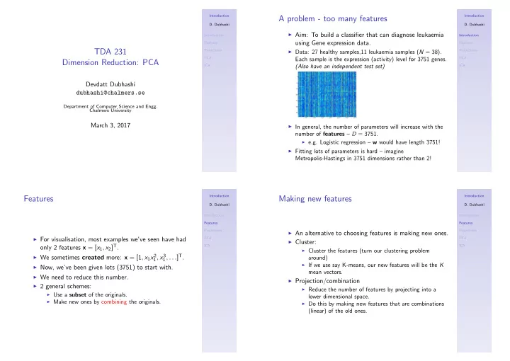
◮ Aim: To build a classifier that can diagnose leukaemia

using Gene expression data.

◮ Data: 27 healthy samples,11 leukaemia samples (N = 38).

Each sample is the expression (activity) level for 3751 genes. (Also have an independent test set)

◮ In general, the number of parameters will increase with the

number of features – D = 3751.

◮ e.g. Logistic regression – w would have length 3751!

◮ Fitting lots of parameters is hard – imagine

Metropolis-Hastings in 3751 dimensions rather than 2!

Introduction

  • D. Dubhashi

Introduction Features Projections PCA ICA

Features

◮ For visualisation, most examples we’ve seen have had

  • nly 2 features x = [x1, x2]T.

◮ We sometimes created more: x = [1, x1x2 1, x3 1, . . .]T. ◮ Now, we’ve been given lots (3751) to start with. ◮ We need to reduce this number. ◮ 2 general schemes:

◮ Use a subset of the originals. ◮ Make new ones by combining the originals. Introduction

  • D. Dubhashi

Introduction Features Projections PCA ICA

Making new features

◮ An alternative to choosing features is making new ones. ◮ Cluster:

◮ Cluster the features (turn our clustering problem

around)

◮ If we use say K-means, our new features will be the K

mean vectors.

◮ Projection/combination

◮ Reduce the number of features by projecting into a

lower dimensional space.

◮ Do this by making new features that are combinations

(linear) of the old ones.

slide-2
SLIDE 2

Introduction

  • D. Dubhashi

Introduction Features Projections PCA ICA

Projection

A 3-dimensional

  • bject

A 2-dimensional projection

Introduction

  • D. Dubhashi

Introduction Features Projections PCA ICA

Projection

◮ We can project data (D dimensions) into a lower

number of dimensions (M).

◮ Z = XW

◮ X is N × D ◮ W is D × M

◮ Z is N × M – an M-dimensional representation of our

N objects.

◮ W defines the projection

◮ Changing W is like changing where the light is coming

from for the shadow (or rotating the hand).

◮ (X is the hand, Z is the shadow)

◮ Once we’ve chosen W we can project test data into this

new space too: Znew = XnewW

Introduction

  • D. Dubhashi

Introduction Features Projections PCA ICA

Choosing W

◮ Different W will give us different projections (imagine

moving the light).

◮ Which should we use? ◮ Not all will represent our data well...

This doesn't look like a hand!

Introduction

  • D. Dubhashi

Introduction Features Projections PCA ICA

Principal Components Analysis

◮ Principal Components Analysis (PCA) is a method for

choosing W.

◮ It finds the columns of W one at a time (define the mth

column as wm).

◮ Each D × 1 column defines one new dimension.

◮ Consider one of the new dimensions (columns of Z):

zm = Xwm

◮ PCA chooses wm to maximise the variance of zm

1 N

N

  • n=1

(zmn − µm)2, µm = 1 N

N

  • n=1

zmn

◮ Once the first one has been found, the w2 is found that

maximises the variance and is orthogonal to the first

  • ne etc etc.
slide-3
SLIDE 3

Introduction

  • D. Dubhashi

Introduction Features Projections PCA ICA

PCA – a visualisation

−3 −2 −1 1 2 3 −3 −2 −1 1 2 3

x1 x2

◮ Original data in 2-dimensions. ◮ We’d like a 1-dimensional projection.

Introduction

  • D. Dubhashi

Introduction Features Projections PCA ICA

PCA – a visualisation

−3 −2 −1 1 2 3 −3 −2 −1 1 2 3 σ2

z = 0.39

x1 x2

◮ Pick some arbitrary w. ◮ Project the data onto it. ◮ Compute the variance (on the line). ◮ The position on the line is our 1 dimensional

representation.

Introduction

  • D. Dubhashi

Introduction Features Projections PCA ICA

PCA – a visualisation

−3 −2 −1 1 2 3 −3 −2 −1 1 2 3 σ2

z = 0.39

x1 x2

σ2

z = 1.2

σ2

z = 1.9

◮ Pick some arbitrary w. ◮ Project the data onto it. ◮ Compute the variance (on the line). ◮ The position on the line is our 1 dimensional

representation.

slide-4
SLIDE 4

Introduction

  • D. Dubhashi

Introduction Features Projections PCA ICA

PCA – analytic solution

◮ Could search for w1, . . . , wM ◮ But, analytic solution is available. ◮ w are the eignvectors of the covariance matrix of X. ◮ Matlab: princomp(x)

Introduction

  • D. Dubhashi

Introduction Features Projections PCA ICA

PCA – analytic solution

−3 −2 −1 1 2 3 −3 −2 −1 1 2 3 σ2

z = 1.9

x1 x2

◮ What would be the second component?

Introduction

  • D. Dubhashi

Introduction Features Projections PCA ICA

PCA – leukaemia data

−40 −20 20 40 −30 −20 −10 10 20

z1 z2

First two principal components in our leukaemia data (points labeled by class).

Introduction

  • D. Dubhashi

Introduction Features Projections PCA ICA

PCA – leukaemia data

5 10 15 20 25 30 0.02 0.04 0.06 0.08 0.1 0.12 M Test error

Test error as more and more components are used.

slide-5
SLIDE 5

Introduction

  • D. Dubhashi

Introduction Features Projections PCA ICA

Summary

◮ Sometimes we have too much data (too many

dimensions).

◮ Features can be dimensions that already exist. ◮ Or we can make new ones.

Introduction

  • D. Dubhashi

Introduction Features Projections PCA ICA

Part 2: ICA (the cocktail party problem)

Introduction

  • D. Dubhashi

Introduction Features Projections PCA ICA

The cocktail party problem

Microphone 2 Microphone 1 Microphone 3 Microphone 4

◮ Each microphone will record a combination of all

speakers.

◮ Can we separate them back out again?

Introduction

  • D. Dubhashi

Introduction Features Projections PCA ICA

Demo

◮ Online: ◮ http://www.cis.hut.fi/projects/ica/cocktail/

cocktail_en.cgi

◮ Matlab:

◮ Available on course webpage ◮ To run: ◮ load ica demo.mat ◮ ica image

slide-6
SLIDE 6

Introduction

  • D. Dubhashi

Introduction Features Projections PCA ICA

Independent components analysis – how it works...

◮ Corrupted data (images/sounds) is a vector of D

  • numbers. i.e. nth image:

xn

◮ We have N images – stack them up into an N × D

matrix: X

◮ Assume that this is the result of the following

corrupting process: X = AS + E

◮ A is mixing matrix. E is noise. (S is N × D).

end ∼ N(0, σ2)

Introduction

  • D. Dubhashi

Introduction Features Projections PCA ICA

Inference

◮ From Bayes’ (look back...)

p(S|X, A, σ2) ∝ p(X|S, A, σ2)p(S)

◮ In our demo, we found values of S, A and σ2 that

maximised the log posterior.

◮ MAP solution... ◮ There is some further reading on the webpage if you

want to know more...

Introduction

  • D. Dubhashi

Introduction Features Projections PCA ICA

Aside – ICA and the central limit theorem

◮ Central limit theorem (paraphrased):

◮ If we keep adding the outcomes of independent random

variables together, we eventually get something that looks Gaussian.

◮ Example: Roll a die m times and take the average.

(Repeat this lots of times to get histogram)

1 2 3 4 5 6 50 100 150 200 Average roll 1 2 3 4 5 6 50 100 150 200 Average roll 1 2 3 4 5 6 50 100 150 200 250 Average roll

◮ From left to right: m = 1, m = 2, m = 5. Looking

more Gaussian as m increases.

Introduction

  • D. Dubhashi

Introduction Features Projections PCA ICA

Aside – ICA and the central limit theorem

◮ Sometimes ICA is performed by reversing this theorem:

X = AS + E

◮ X is some random variables added together. ◮ It will be more ‘Gaussian’ than S ◮ Find S that is as non-Gaussian as possible. ◮ More resource:

◮ http://www.cis.hut.fi/projects/ica/icademo/ ◮ http://www.cis.hut.fi/projects/ica/

slide-7
SLIDE 7

Introduction

  • D. Dubhashi

Introduction Features Projections PCA ICA

Summary

◮ PCA and ICA are both examples of projection

techniques.

◮ Both assume a linear transformation

◮ ICA: X = AS + E ◮ PCA: Z = XW

◮ PCA can be used for Data pre-processing or

visualisation.

◮ ICA can be used to separate sources that have been

mixed together.

◮ Also looked at PCA as a feature selection method.