a i a j Input Input Activation Output Output Links Function - - PowerPoint PPT Presentation

▶

Nov 25, 2023 283 likes •351 views

Neural Learning Methods } An obvious source of biological inspiration for learning research: the brain } The work of McCulloch and Pitts on the perceptron (1943) started as research into how we could precisely model the neuron and the network of

SLIDE 1

1

Class #19: Neural Networks

Machine Learning (COMP 135): M. Allen, 30 March 20

1

Neural Learning Methods

} An obvious source of biological inspiration for learning

research: the brain

} The work of McCulloch and Pitts on the perceptron

(1943) started as research into how we could precisely model the neuron and the network of connections that allow animals (like us) to learn

} These networks are used as classifiers: given an input,

they label that input with a classification, or a distribution

ver possible classifications

Monday, 30 Mar. 2020 Machine Learning (COMP 135) 2

2

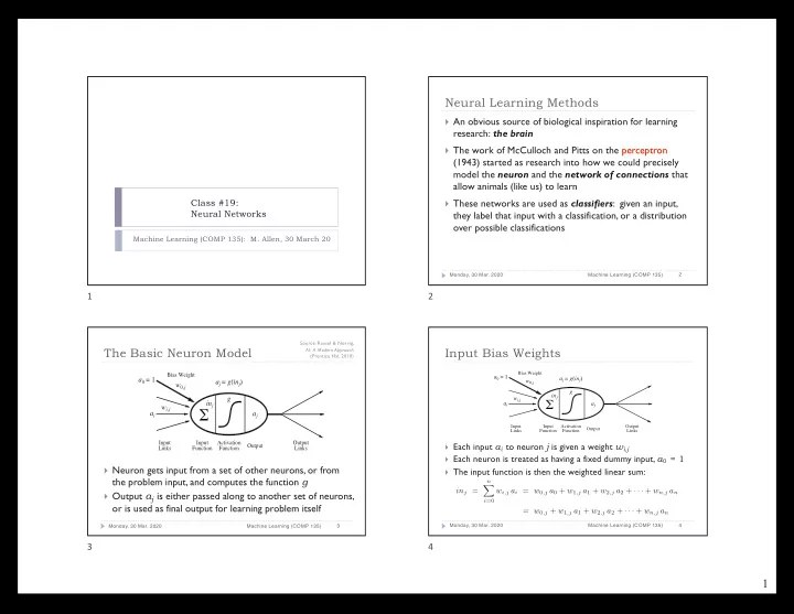
The Basic Neuron Model

} Neuron gets input from a set of other neurons, or from

the problem input, and computes the function g

} Output aj is either passed along to another set of neurons,

r is used as final output for learning problem itself

Monday, 30 Mar. 2020 Machine Learning (COMP 135) 3

Output

Σ

Input Links Activation Function Input Function Output Links

a0 = 1 aj = g(inj) aj g inj wi,j w0,j

Bias Weight

ai

Source: Russel & Norvig, AI: A Modern Approach (Prentice Hal, 2010)

3

Input Bias Weights

} Each input ai to neuron j is given a weight wi,j } Each neuron is treated as having a fixed dummy input, a0 = 1 } The input function is then the weighted linear sum:

Monday, 30 Mar. 2020 Machine Learning (COMP 135) 4 Output

Σ

Input Links Activation Function Input Function Output Links

a0 = 1 aj = g(inj) aj g inj wi,j w0,j

Bias Weight

inj =

X

i=0

wi,j ai = w0,j a0 + w1,j a1 + w2,j a2 + · · · + wn,j an = w0,j + w1,j a1 + w2,j a2 + · · · + wn,j an

4

SLIDE 2

2 We’ve Seen This Before!

} The weighted linear sum of inputs, with dummy, a0 = 1, is just a form

f the cross-product that our classifiers have been using all along

} Remember that the “neuron” here is just another way of looking at the

perceptron idea we already discussed

Monday, 30 Mar. 2020 Machine Learning (COMP 135) 5 Output

Σ

Input Links Activation Function Input Function Output Links

a0 = 1 aj = g(inj) aj g inj wi,j w0,j

Bias Weight

inj =

X

i=0

wi,j ai = w0,j + w1,j a1, +w2,j a2 + · · · + wn,j an = wj · a

5

Neuron Output Functions

} While the inputs to any neuron are treated in a linear

fashion, the output function g need not be linear

} The power of neural nets comes from fact that we can

combine large numbers of neurons together to compute any function (linear or not) that we choose

Monday, 30 Mar. 2020 Machine Learning (COMP 135) 6 Output

Σ

Input Links Activation Function Input Function Output Links

a0 = 1 aj = g(inj) aj g inj wi,j w0,j

Bias Weight

6

The Perceptron Threshold Function

} One possible function is the binary threshold, which is

suitable for “firm” classification problems, and causes the neuron to activate based on a simple binary function:

Monday, 30 Mar. 2020 Machine Learning (COMP 135) 7 Output

Σ

Input Links Activation Function Input Function Output Links

a0 = 1 aj = g(inj) aj g inj wi,j w0,j

Bias Weight

g(inj) = ( 1 if inj ≥ 0 else

7

The Sigmoid Activation Function

} A function that has been more often used in neural networks is

the logistic (also known as the Sigmoid), as seen before

} This gives us a “soft” value, which we can often interpret as the

probability of belonging to some output class

Monday, 30 Mar. 2020 Machine Learning (COMP 135) 8 Output

Σ

Input Links Activation Function Input Function Output Links

a0 = 1 aj = g(inj) aj g inj wi,j w0,j

Bias Weight

g(inj) = 1 1 + e−inj

8

SLIDE 3

3 Power of Perceptron Networks

} A single-layer network combines a linear function of input

weights with the non-linear output function

} If we threshold output, we have a boolean (1/0) function } This is sufficient to compute numerous linear functions

Monday, 30 Mar. 2020 Machine Learning (COMP 135) 9

x1 x2 y 1 1 1 1 1 1 1

x1 OR x2

x1 x2 y 1 1 1 1 1

x1 AND x2

9

Power of Perceptron Networks

} A single-layer network with inputs for variables (x1, x2), and

bias term (x0 == 1), can compute OR of inputs

} Threshold: (y == 1) if weighted sum (S >= 0); else (y == 0)

} What weights can we apply to the three inputs to produce OR?

} One answer: -0.5 + x1 + x2

Monday, 30 Mar. 2020 Machine Learning (COMP 135) 10

x1 x2 y 1 1 1 1 1 1 1

x1 OR x2

1 x1 x2

y

10

Power of Perceptron Networks

} What about the AND function instead?

} One answer: -1.5 + x1 + x2

Monday, 30 Mar. 2020 Machine Learning (COMP 135) 11

x1 x2 y 1 1 1 1 1

x1 AND x2

1 x1 x2

y

11

Linear Separation with Perceptron Networks

} We can think of binary functions as dividing (x1, x2) plane } The ability to express such a function is analogous to the ability

to linearly separate data in such regions

Monday, 30 Mar. 2020 Machine Learning (COMP 135) 12

x2 x1 1 1

= 0 = 1

x1 x2 y 1 1 1 1 1 1 1

x1 OR x2

12

SLIDE 4

4 Linear Separation with Perceptron Networks

} We can think of binary functions as dividing (x1, x2) plane } The ability to express such a function is analogous to the ability

to linearly separate data in such regions

Monday, 30 Mar. 2020 Machine Learning (COMP 135) 13

x2 x1 1 1

= 0 = 1

x1 x2 y 1 1 1 1 1

x1 AND x2

13

Functions with Non-Linear Boundaries

}

There are some functions that cannot be expressed using a single layer of linear weighted inputs, and a non-linear output

}

Again, this is analogous to the inability to linearly separate data in some cases

Monday, 30 Mar. 2020 Machine Learning (COMP 135) 14

= 0 = 1

x1 x2 y 1 1 1 1 1 1

x1 XOR x2

x2 x1 1 1

14

MLP’s for Non-Linear Boundaries

} Neural networks gain expressive power

because they can have more than one layer

} A multi-layer perceptron has one or more

hidden layers between input and output

} Each hidden node applies a non-linear

activation function, producing output that it sends along to the next layer

}

In such cases, much more complex functions are possible, corresponding to non-linear decision boundaries (as in current homework assignment)

Monday, 30 Mar. 2020 Machine Learning (COMP 135) 15

x2 x1 1 1

1 x1 x2

y

h1 h2

15

Review: Properties of the Sigmoid Function

} The Sigmoid takes its name

from the shape of its plot

} It always has a value in range:

0 ≤ x ≤ 1

} The function is everywhere

differentiable, and has a derivative that is easy to calculate, which turns out to be useful for learning:

Monday, 30 Mar. 2020 Machine Learning (COMP 135) 16

g(inj) = 1 1 + e−inj

8 0.5 1

6 -4 -2 0

2 4 6

(b)

g0(inj) = g(inj)(1 − g(inj))

16

SLIDE 5

5 Do We Always Use the Logistic Sigmoid?

} While historically popular, the logistic function is not always

used in modern neural network research

} There are many other functions that can be, and are, used } Some models even use combinations of different functions on

different layers of the network

} Often, the logistic is used at the final layer only, where it is

sometimes called a softmax (probability) function

} In our presentation, we will assume the logistic, but the overall

details of the key algorithm do not change if we use something else

} In general, we want a function that is

Non-linear: allowing for more complex outputs.

Differentiable: standard back-propagation algorithms for learning in the networks use gradient-based approaches, and require access to the derivative of the function

Monday, 30 Mar. 2020 Machine Learning (COMP 135) 17

17

Other Popular Activation Functions

Monday, 30 Mar. 2020 Machine Learning (COMP 135) 18

} The rectifier (or “ramp”) function is popular for many modern applications

}

A network using the rectifier is known as a rectifier linear unit (ReLU)

} The Softplus function is a smooth approximation to the rectifier

5
4.75
4.5
4.25
4
3.75
3.5
3.25
3
2.75
2.5
2.25
2
1.75
1.5
1.25
1
0.75
0.5
0.25

0.25 0.5 0.75 1 1.25 1.5 1.75 2 2.25 2.5 2.75 3 3.25 3.5 3.75 4 4.25 4.5 4.75 5 RELU Softplus

RELU(x) = max(0, x)

Softplus(x) = ln(1 + ex)

18

Other Popular Activation Functions

Monday, 30 Mar. 2020 Machine Learning (COMP 135) 19

} The ReLU function has

derivative:

} For many purposes, the

undefined value of the derivative is simply set arbitrarily (say to 0.5)

5
4.75
4.5
4.25
4
3.75
3.5
3.25
3
2.75
2.5
2.25
2
1.75
1.5
1.25
1
0.75
0.5
0.25

0.25 0.5 0.75 1 1.25 1.5 1.75 2 2.25 2.5 2.75 3 3.25 3.5 3.75 4 4.25 4.5 4.75 5 RELU Softplus

RELU(x) = max(0, x)

Softplus(x) = ln(1 + ex)

} Alternatively, if using Softplus approximation, we have a well-defined

derivative everywhere:

δ ReLU δx (x) =      if input x < 0 1 if input x > 0 undef if input x = 0

<latexit sha1_base64="q/mgLMLH2nu2384xKtztQ4KCrv0=">ACi3icbVFNaxRBEO0Zv+KYmFUPIl4KgxIhLDObg0E3EhTBg4cobhJIL0tPT82mSW/30FMTNgzd/w54lUvXv0Z9s6OhzUpaCje/XRr9JCq5Li+GcQ3rh56/adtbvRvfWN+5u9Bw+PSls5iSNptXUnqShRK4MjUqTxpHAoZqnG4/T8/YI/vkBXKmu+0mWB45mYGpUrKchDk943njsha56hJsF3gBPOqf6Cn0ZN06Ewb7bnL2EfIp7iVJla+nlEwHE8KIrUDkoU1QEDcxh6AnOPZ9cz7/9x1cmw/x6zT7EUeTdcMmva24H7cBV5OkS7YO9n7/ePzrz5PDSe87z6ysZmhIalGWp0lc0LgWjpTU2ES8KrEQ8lxMsW5dbOC5hzLIrfPELTois5Yal1bqT6tKN8b1+3maOSyTV5pIAsLwyFTDiXpS58I6ZSfD/JMeNPJn2Wlk6s0Zjtwsbhl5nfVU+v1Z7OB39cbkPz/3avJ0aCf7PYHn70T79gy1thT9oxts4S9YgfsIztkIyaD9WAQvAmG4Ua4G74Oh0tpGHQ1j9hKhB/+AsFWw6Q=</latexit>

δ Softplus δx (x) = 1 1 + e−x

<latexit sha1_base64="IBb/29IkMtbjRdINiEIbY0j1BMg=">ACKXicZVDLSgNBEJz1GeMr6tHLoAiKGnaTg4IQT14jGhUcGOYzPYmQyY7y2yvRJYFv0f/xcfNBMGDP+LkcYkWDBTd1T1dVQ+liNC2u9bE5NT0zGxmLju/sLi0nFtZvY5UrDlUuJK39ZBFIEUEGBEm5Daxdl3BTb532+zcPoCOhgit8DKHaZo1A+IzNKVa7sz1NeOJ64FE5u5RF6GDyaXyMZRxlKajDu2k250dekzpUO+kiUN3Kdwn+50reU27bw9AP1PnBHZLB19vz19FXW5lnt1PcXjNgTIJYuiO8cOsZowjYJLSLNuHEHIeIs1IBl4TOmWKXnUV9q8AOmgOqYLFA48jU3fxegfVhMRhDFCwIdr/FhSVLQfB/WEBo7y0RDGtTD/U95kxiKa0MY26ViCt0cf+kl75lbZUEbfbBfMvSYA56/d/+S6kHeK+cKFSeKEDJEh62SDbBOHJASOSdlUiGcPJN30iU968X6sD6t3lA6Y1m1sgYrJ9fDimq9Q=</latexit>

The derivative of Softplus is the Sigmoid Logistic!

19

Activation Functions Everywhere!

} Logistic } ReLU } Softplus } Hyperbolic

Tangent

} Gaussian

Monday, 30 Mar. 2020 Machine Learning (COMP 135) 20

f(x) = 1 1 + e−x

<latexit sha1_base64="/7q+CwPyrfTqTN0sDWcV5uZlYw=">ACAXicZVDLSsNAFJ3UV62vqEtdDBahopakXSiIUHTjsoJ9QFvLZDJph04yYTIpLSEg+jO60279B10Lgr/iNO0memDgcOY+zj2Wz2gDeNLywsLi2vZFdza+sbm1v69k494KHApIY546JpoYAw6pGapJKRpi8Ici1GtbgevrfGBIRUO7dybFPOi7qedShGEkldfV9pzA6gpcQth2BcGTGkQmPIbmPTkdx3NXzRtFIAP8Tc07ylYufz4fvsqh29Y+2zXHoEk9ihoKgZRq+7ERISIoZiXPtMCA+wgPUI1HiPYaHSrKhw4V6noSJmqrzuEy8prpboXTOxH1/FASD8/GOCGDksPpmdCmgmDJxogLKjaD3EfqROlCiM1SYSM2CdwOE3QVl5Zj6v6vltSflUA5t9z/5N6qWiWi6VblcQVmCEL9sABKATnIEKuAFVUAMYPIJn8AYm2pP2or1qk1lpRpv37IUtPdfNy6ZXg=</latexit>

δf δx(x) = f(x)(1 − f(x))

<latexit sha1_base64="M7pK/4noCUYEJXzWCjGmZQXRdo0=">ACE3icZVBNT8IwGO7wC/Fr6sEYL43EBIlGx7kYkL04hETARNGSNd10FDWpesIZNm/0D+jN+Wq8aoXr/4My8D5EmaPn7vG/f57F9RgNpGJ9aZml5ZXUtu57b2Nza3tF39xoBDwUmdcwZF/c2CgijHqlLKhm59wVBA5uRpt2/nr43h0QElHt3cuyT9gB1PepSjKQqdfS5QqEI8shTCLoxn9sFBdGRXgJoavugnPElLs6HmjZCSAi8Sck3y18v1x8PVzWOvo75bDcTgnsQMBUHLNHzZjpCQFDMS56wID7CfdQlUeImhieq5ECXC3U8CZNqSudxmWyf6m6F0q20I+r5oSQeno1xQwYlh1Pj0KGCYMnGiAsqPof4h5S5qWKJzVJhIw4p3A4zdRu7IuV/reoKz2VQGY/+0uka5ZJ6XyrcqiSswQxYcgWNQACa4AFVwA2qgDjB4AE/gFUy0R+1Ze9EmM2lGm/fsgxS0t186hJ+l</latexit>

f(x) = max(0, x)

<latexit sha1_base64="16vpD/wm4aoVI8uPj4SV3wehX0c=">AB93icZVDLTsJAFJ3iC/FVcelmAjGBSEiLC92YEN24xEQeCSVkOp3ChOlM50SGsJfuNadsvVH3PM3DoVN5SaTnJw595zjxsyGinLWhm5vf2Dw6P8ceHk9Oz8wrwsdiIRS0zaWDAhey6KCKOctBVjPRCSVDgMtJ1J8/r/+6UyIgK/qaSkAwCNOLUpxgpTQ3Nol+ZVeEjhE6AZhWrBmfVoVm26lZacBfYW1Bulpzb91UzaQ3NX8cTOA4IV5ihKOrbVqgGcyQVxYwsCk4ckRDhCRqRep4AW805UFfSP24gimb0XGhUoeZ7n6s/IfBnPIwVoTjzRg/ZlAJuD4OelQSrFiAcKS6v0Qj5FEWOkIMpNkzIhXg9N1bp72ykZC68dBQ/vVAdj/z90FnUbdvqs3XnUST2BTeXANSqACbHAPmuAFtEAbYDADH+AbLI3E+DS+jOVGmjO2PVcgU8bPH729k7E=</latexit>

δf δx(x) = {0, undef, 1}

<latexit sha1_base64="5N8Wax2x/07v2Q6gCfzYLms+Js=">ACGnicZVDLSgMxFM34tr6qLkTcBEVQKGWmInYjiG5cKtgqOKWkmTs1NE2GzJ3SMsyX6M/oTgVx4UY3bv0M01YX1QOBw8l9ndOIpIjRd+dsfGJyanpmdnc3PzC4lJ+eaUa68RwqHAtblqsBikUFBgRKuIgOs3ZBw2Wid9P8vO2BiodUF9iKotVlTiVBwhlaq5/f90DCe+gFIZDTMflk32+nu0kNK/RgwdQt+gSYqgLBPvKye3KL7gD0P/F+yNZR+fN17eNr/ayef/EDzZM2KOSxfG150ZYS5lBwSVkOT+JIWK8xZqQDkxldNtKAQ21sU8hHagjdUrjwMRI93WCYbmWChUlCIoPx4SJpKhp3z8NhAGOsmcJ40bY/ZTfMJsB2pRGJplEQlCgnX60gb1VNrWtv2mX7L02AO+v3f+kWip6e8XSuU3imAwxQzbIJtkhHjkgR+SUnJEK4eSW3JMn8uzcOQ/Oo/M8LB1zfnpWyQict2/lC6NZ</latexit>

f(x) = ln(1 + ex)

<latexit sha1_base64="q8uHaxZfwBNXlAHFxSd5nNSsdE=">AB+XicZVDLTgIxFO3gC/E1PnZuGogJBENmcKEbE6Ibl5jI2GQdDodaOi0k06HgIS/8AN0p2z9D/f8jWVgM3KTJien5957nFDRiNlWQsjs7W9s7uX3c8dHB4dn5inZ81IxBKTBhZMyLaLIsIoJw1FSPtUBIUuIy03OHj8r81IjKigr+oSUi6Aepz6lOMlKZ65oVfHJfgPYQO40UbliF5HZd6ZsGqWEnBTWCvQaGWd8rvi9qk3jN/HU/gOCBcYaiqGNboepOkVQUMzLOXFEQoSHqE+miecZvNKUB30h9eMKJmxKx4VKPKa6O7Hy7pTysNYEY5XY/yYQSXg8jzoUmwYhMNEJZU74d4gCTCSoeQmiRjRrxrOFom52mvrC+0fhBUtV8dgP3/3E3QrFbsm0r1WSfxAFaVBZcgD4rABregBp5AHTQABm/gA3yDuTE1Po0vY76SZox1zlIlfHzB8JklDw=</latexit>

δf δx(x) = 1 1 + e−x

<latexit sha1_base64="aypNpyJDLZ5/AHeipvXf4M8jg=">ACGXicZVBbSwJBGJ21m9nN6rGXIQmMSnY1KIhA6qVHg7yAmoyz3+rguLPMzoqyLPQ76s/UW/lQDz0FQX+l8dKDeWDgcL7LfOc0Pc58ZpfRmxhcWl5Jb6aWFvf2NxKbu+UfBFICkUquJCVJvGBMxeKikOFU8C6TY5lJud61G93APpM+HeqYEH9S5pucxhlCgtNZKnNUcSGtZs4IpgJ/pj/SjdP8SXGE/qVhRa+AjDfXjSj6JGMmVmzDHwPLGmJW/+Pl4+M7JQiP5XrMFDbrgKsqJ71ct01P1kEjFKIcoUQt8AjtkBaEY08RPtCSjR0h9XMVHqszfa5QYw8z09VAOef1kLleoMClkzVOwLESeGQf20wCVXygCaGS6f8xbRNtUemQZjbJgIN9jHujZG19K28J3d/uZvW9OgDrv915UspmrFwme6uTuEITxNEe2kdpZKEzlEc3qICKiKJH9Ize0NB4Ml6MV2M4aY0Z05ldNAPj8xdOFKO6</latexit>

f(x) = 1 − e−2x 1 + e−2x

<latexit sha1_base64="5CY3krbDCxyS+0yrvt5TX46KzY=">ACDHicZVBNSwJBGJ61L7Mvq2OXIYmMSnb1UBCB1KWjQX6Amoyzszo4O7PMzoqyLPQH6s/Urbx2rHMQ9FcaVwnMFwae95n363naHqO+Ms0vI7GwuLS8klxNra1vbG6lt3cqvgkJmUsmJC1NvIJo5yUFVWM1DxJkNtmpNruXY/q30ifSr4nRp6pOmiDqcOxUhpqpU+dLKDI3gJYcORCIcWPIXkPjzND6JIJ8d/SudMXNmHAeWFOQKV78fD58F2Splf5o2AIHLuEKM+T7dcv0VDNEUlHMSJRqBD7xEO6hDgljGRE80JQNHSH14wrG7EwdFyo+e6a7HijnvBlS7gWKcDwZ4wQMKgHiqFNJcGKDTVAWFK9H+Iu0mqV9mVmkgwYsU9gf2ymrW9lHaHru25e36sNsP7LnQeVfM4q5PK32okrMIk2AP7IAscAaK4AaUQBlg8AiewRsYGU/Gi/FqjCalCWPaswtmwnj/BQOnP0=</latexit>

δf δx(x) = 1 − f(x)2

<latexit sha1_base64="ea7ayQsKpRhFLZLFYzefjaQSU4k=">ACD3icZVBJSwMxGM3UrdZt1IOIl2ARqmiZGQ/2IhS9eKxgF2hrSTOZNjSTDJlMaRn6H/TP6E179SJe9eLVn2G6eKh9EHi8fNt7zYDRUFnWp5FYWFxaXkmuptbWNza3zO2dUigiUkRCyZkpYlCwignRUVI5VAEuQ3GSk3O9ej/3KXyJAKfqf6Aan7qMWpRzFSWmqYJzVPIhzXMIUgt7gj/UGmd4xvITQhmfQ0/zeaZhpK2uNAeJPSXpfO7Y+/rZ7/QMN9rsCRT7jCDIVh1bYCVY+RVBQzMkjVopAECHdQi8RjJwN4pCUXekLqxUcqzN1XKjx5TPd1Uh5uXpMeRApwvFkjBcxqAQcmYulQr1tcEYUn1fojbSBtXOpqZSTJixD2F3VGer6VtYSub/uOvlcHYP+3O09KTtY+zq3OokrMESHIBDkAE2uAB5cAMKoAgweABP4BUMjUfj2XgxhpPShDHt2QUzMN5+AQMpno0=</latexit>

δf δx(x) = −x f(x)

<latexit sha1_base64="zcLM/mtpT2rJcgDnbrn0QZozgqo=">ACDnicZVC7TsMwFHXKq5RXgQEhFosKqZVKlZSBLkgVLIxFog+pqSrHcVqrThw5TtUqyjfAz8AGXZkQKysfAbugyH0SpaOj+9PudYPqOB1PVPLbWyura+kd7MbG3v7O5l9w8aAQ8FJnXMGRctCwWEUY/UJZWMtHxBkGsx0rQGN9P35pCIgHLvXo590nFRz6MOxUgqpstmI5AODJtwiSCTvyHRnF+VIBXEJ6PzCJ01KWbzeklfVZwGRgLkKtWvj+Ovn6Oa93su2lzHLrEk5ihIGgbui87ERKSYkbijBkGxEd4gHokmhmJ4ZmibOhwoY4n4YxN9HlczoQnptuhdCqdiHp+KImH52uckEHJ4dQztKkgWLKxAgLqv6HuI+Ub6mSWwSISN2EQ6ncdpK+tx1d93y0qvCsD4b3cZNMol46JUvlNJXIN5pcEJOAV5YIBLUAW3oAbqAIMH8ARewUR71J61F20yb01pi5lDkCjt7RcB5p6i</latexit>

f(x) = e− x2

<latexit sha1_base64="tRe7RD6O2cNXBy1rjIj3O6KEDls=">AB/3icZVDLTsJAFJ3iC/FVdaebCcQEo5K2LnRjQnTjEhN5JBTIdDqFCdNOM50SNE/8Fv0J2y9Sfc8zcOhQ16klOztzHucJGY2kYcy03Nr6xuZWfruws7u3f6AfHjUiHgtM6pgzLloOigijAalLKhlphYIg32Gk6Qwf5v/NERER5cGznISk46N+QD2KkVRSTz/xyuNzeAch6SZXticQTsZdK02sNO3pJaNiZID/ibkpWrRvnibVSe1nv5juxzHPgkZiK2qYRyk6ChKSYkbRgxEJER6iPky5yk8U5ILPS7UCyTM1JW6gMvM6Up3O5bebSehQRhLEuDFGC9mUHI4PxK6VBAs2UQRhAV+yEeIHWcVFGsTBIxI+4lHM3zc5VX1ueqfuBbyq8KwPx7n/SsCrmdcV6UkncgwXy4BQUQRmY4AZUwSOogTrA4AW8gy8w1V61D+1Tmy5Kc9qy5xisQPv+BVXpmCQ=</latexit>

20

SLIDE 6

6 Choosing Activation Functions

Monday, 30 Mar. 2020 Machine Learning (COMP 135) 21

} Functions have different pros and cons: 1.

Sigmoid: historically popular, less so today

} Susceptible to saturation: very large weights, tiny gradients } Not zero-centered, which is sometimes inconvenient } More popular as an output probability function (softmax) 2.

Hyperbolic tangent

} Can saturate like the sigmoid, but is zero-centered 3.

ReLU/Softplus: most popular function in modern uses

} ReLU is susceptible to “dying” neurons (these do not

contribute to output in any real way)

} Sensitive to learning rate } Softplus sometimes preferred, due to its smoothness