A C Standard model has 1-1 correspondence between symbols and - - PDF document

SLIDE 1

CSCE 471/871 Lecture 3: Markov Chains and Hidden Markov Models

Stephen D. Scott

1

Outline

• Markov chains
• Hidden Markov models (HMMs)

– Formal definition – Finding most probable state path (Viterbi algorithm) – Forward and backward algorithms

• Specifying an HMM

2

Markov Chains An Example: CpG Islands

• Focus on nucleotide sequences
• The sequence “CG” (written “CpG”) tends to appear more frequently

in some places than in others

• Such CpG islands are usually 102–103 bases long
• Questions:
• 1. Given a short segment, is it from a CpG island?
• 2. Given a long segment, where are its islands?

3

Modeling CpG Islands

• Model will be a CpG generator
• Want probability of next symbol to depend on current symbol
• Will use a standard (non-hidden) Markov model

– Probabilistic state machine – Each state emits a symbol

4

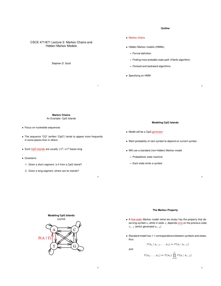
Modeling CpG Islands (cont’d)

A C T G P(A | T)

5

The Markov Property

• A first-order Markov model (what we study) has the property that ob-

serving symbol xi while in state ⇡i depends only on the previous state ⇡i1 (which generated xi1)

• Standard model has 1-1 correspondence between symbols and states,

thus P(xi | xi1, . . . , x1) = P(xi | xi1) and P(x1, . . . , xL) = P(x1)

L Y i=2

P(xi | xi1)

6

SLIDE 2

Begin and End States

• For convenience, can add special “begin” (B) and “end” (E) states to

clarify equations and define a distribution over sequence lengths

• Emit empty (null) symbols x0 and xL+1 to mark ends of sequence

A C T G B E P(x1, . . . , xL) =

L+1 Y i=1

P(xi | xi1)

• Will represent both with single state named 0

7

Markov Chains for Discrimination

• How do we use this to differentiate islands from non-islands?
• Define two Markov models: islands (“+”) and non-islands (“”)

– Each model gets 4 states (A, C, G, T) – Take training set of known islands and non-islands – Let c+

st = number of times symbol t followed symbol s in an island:

ˆ P +(t | s) = c+

st P t0 c+ st0

• Example probabilities in [Durbin et al., p. 51]
• Now score a sequence X = hx1, . . . , xLi by summing the log-odds ratios:

log

ˆ

P(X | +) ˆ P(X | )

!

=

L+1 X i=1

log

ˆ

P +(xi | xi1) ˆ P (xi | xi1)

!

8

Outline

• Markov chains
• Hidden Markov models (HMMs)

– Formal definition – Finding most probable state path (Viterbi algorithm) – Forward and backward algorithms

• Specifying an HMM

9

Hidden Markov Models

• Second CpG question: Given a long sequence, where are its islands?

– Could use tools just presented by passing a fixed-width window

• ver the sequence and computing scores

– Trouble if islands’ lengths vary – Prefer single, unified model for islands vs. non-islands

A + C T G + + + A C T G

• between all pairs]

[complete connectivity

– Within the + group, transition probabilities similar to those for the separate + model, but there is a small chance of switching to a state in the group

10

What’s Hidden in an HMM?

• No longer have one-to-one correspondence between states and emit-

ted characters – E.g. was C emitted by C+ or C?

• Must differentiate the symbol sequence X from the state sequence

⇡ = h⇡1, . . . , ⇡Li – State transition probabilities same as before: P(⇡i = ` | ⇡i1 = j) (i.e. P(` | j)) – Now each state has a prob. of emitting any value: P(xi = x | ⇡i = j) (i.e. P(x | j))

11

What’s Hidden in an HMM? (cont’d) [In CpG HMM, emission probs discrete and = 0 or 1]

12

SLIDE 3

Example: The Occasionally Dishonest Casino

• Assume that a casino is typically fair, but with probability 0.05 it switches

to a loaded die, and switches back with probability 0.1

1: 1/6 2: 1/6 3: 1/6 4: 1/6 5: 1/6 6: 1/6 Loaded Fair 1: 1/10 2: 1/10 3: 1/10 4: 1/10 5: 1/10 6: 1/2 0.05 0.1 0.9 0.95

• Given a sequence of rolls, what’s hidden?

13

The Viterbi Algorithm

• Probability of seeing symbol sequence X and state sequence ⇡ is

P(X, ⇡) = P(⇡1 | 0)

L Y i=1

P(xi | ⇡i) P(⇡i+1 | ⇡i)

• Can use this to find most likely path:

⇡⇤ = argmax

⇡

P(X, ⇡) and trace it to identify islands (paths through “+” states)

• There are an exponential number of paths through chain, so how do

we find the most likely one?

14

The Viterbi Algorithm (cont’d)

• Assume that we know (for all k) vk(i) = probability of most likely path

ending in state k with observation xi

• Then

v`(i + 1) = P(xi+1 | `) max

k

{vk(i) P(` | k)} l All states at State at i l +1 i

15

The Viterbi Algorithm (cont’d)

• Given the formula, can fill in table with dynamic programming:

– v0(0) = 1, vk(0) = 0 for k > 0 – For i = 1 to L; for ` = 1 to M (# states) ⇤ v`(i) = P(xi | `) maxk{vk(i 1)P(` | k)} ⇤ ptri(`) = argmaxk{vk(i 1)P(` | k)} – P(X, ⇡⇤) = maxk{vk(L)P(0 | k)} – ⇡⇤

L = argmaxk{vk(L)P(0 | k)}

– For i = L to 1 ⇤ ⇡⇤

i1 = ptri(⇡⇤ i )

• To avoid underflow, use log(v`(i)) and add

16

The Forward Algorithm

• Given a sequence X, find P(X) = P

⇡ P(X, ⇡)

• Use dynamic programming like Viterbi, replacing max with sum, and

vk(i) with fk(i) = P(x1, . . . , xi, ⇡i = k) (= prob. of observed sequence through xi, stopping in state k) – f0(0) = 1, fk(0) = 0 for k > 0 – For i = 1 to L; for ` = 1 to M (# states) ⇤ f`(i) = P(xi | `) P

k fk(i 1)P(` | k)

– P(X) = P

k fk(L)P(0 | k)

• To avoid underflow, can again use logs, though exactness of results

compromised (Section 3.6)

17

The Backward Algorithm

• Given a sequence X, find the probability that xi was emitted by state

k, i.e. P(⇡i = k | X) = P(⇡i = k, X) P(X) =

fk(i) z }| {

P(x1, . . . , xi, ⇡i = k)

bk(i) z }| {

P(xi+1, . . . , xL | ⇡i = k) P(X)

| {z }

computed by forward alg

• Algorithm:

– bk(L) = P(0 | k) for all k – For i = L 1 to 1; for k = 1 to M (# states) ⇤ bk(i) = P

` P(` | k) P(xi+1 | `) b`(i + 1)

18

SLIDE 4

Example Use of Forward/Backward Algorithm

• Define g(k) = 1 if k 2 {A+, C+, G+, T+} and 0 otherwise
• Then G(i | X) = P

k P(⇡i = k | X) g(k) = probability that xi is in

an island

• For each state k, compute P(⇡i = k | X) with forward/backward

algorithm

• Technique applicable to any HMM where set of states is partitioned

into classes – Use to label individual parts of a sequence

19

Outline

• Markov chains
• Hidden Markov models (HMMs)

– Formal definition – Finding most probable state path (Viterbi algorithm) – Forward and backward algorithms

• Specifying an HMM

20

Specifying an HMM

• Two problems: defining structure (set of states) and parameters (tran-

sition and emission probabilities)

• Start with latter problem, i.e. given a training set X1, . . . , XN of inde-

pendently generated sequences, learn a good set of parameters ✓

• Goal is to maximize the (log) likelihood of seeing the training set given

that ✓ is the set of parameters for the HMM generating them:

N X j=1

log(P(Xj; ✓))

21

When State Sequence Known

• Estimating parameters when e.g. islands already identified in training

set

• Let Ak` = number of k ! ` transitions and Ek(b) = number of

emissions of b in state k P(` | k) = Ak` /

@X `0

Ak`0

1 A

P(b | k) = Ek(b) /

@X b0

Ek(b0)

1 A

22

When State Sequence Known (cont’d)

• Be careful if little training data available

– E.g. an unused state k will have undefined parameters – Workaround: Add pseudocounts rk` to Ak` and rk(b) to Ek(b) that reflect prior biases about parobabilities – Increased training data decreases prior’s influence – [Sj¨

• lander et al. 96]

23

The Baum-Welch Algorithm

• Used for estimating parameters when state sequence unknown
• Special case of the expectation maximization (EM) algorithm
• Start with arbitrary P(` | k) and P(b | k), and use to estimate Ak`

and Ek(b) as expected number of occurrences given the training set⇤: Ak` =

N X j=1

1 P(Xj)

L X i=1

fj

k(i) P(` | k) P(xj i+1 | `) bj `(i + 1)

(Prob. of transition from k to ` at position i of sequence j, summed

• ver all positions of all sequences)

Ek(b) =

N X j=1 X i:xj

i=b

P(⇡i = k | Xj) =

N X j=1

1 P(Xj)

X i:xj

i=b

fj

k(i) bj k(i)

• Use these (& pseudocounts) to recompute P(` | k) and P(b | k)
• After each iteration, compute log likelihood and halt if no improvement

⇤Superscript j corresponds to jth train example

24

SLIDE 5

HMM Structure

• How to specify HMM states and connections?
• States come from background knowledge on problem, e.g. size-4 al-

phabet, +/, ) 8 states

• Connections:

– Tempting to specify complete connectivity and let Baum-Welch sort it out – Problem: Huge number of parameters could lead to local max – Better to use background knowledge to invalidate some connec- tions by initializing P(` | k) = 0 ⇤ Baum-Welch will respect this

25

Silent States

• May want to allow model to generate sequences with certain parts

deleted – E.g. when aligning DNA or protein sequences against a fixed model

• r matching a sequence of spoken words against a fixed model,

some parts of the input might be omitted

• Problem: Huge number of connections, slow training, local maxima

26

Silent States (cont’d)

• Silent states (like begin and end states) don’t emit symbols, so they

can “bypass” a regular state

• If there are no purely silent loops, can update Viterbi, forward, and

backward algorithms to work with silent states [Durbin et al., p. 72]

• Used extensively in profile HMMs for modeling sequences of protein

families (aka multiple alignments)

27

Topic summary due in 1 week!

28