A Bayesian Approach to Lagrangian Data Assimilation Chris Jones, UNC - PDF document

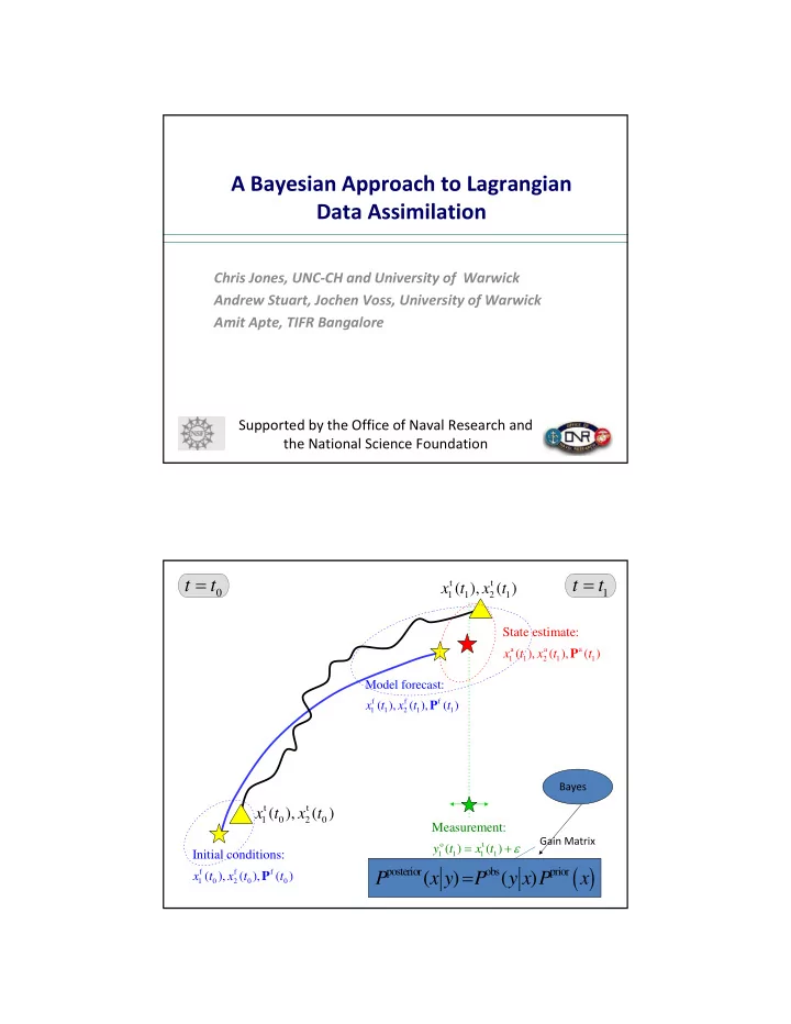
A Bayesian Approach to Lagrangian Data Assimilation Chris Jones, UNC ‐ CH and University of Warwick Andrew Stuart, Jochen Voss, University of Warwick Amit Apte, TIFR Bangalore Supported by the Office of Naval Research and the National Science Foundation = = t t t t t t ( ), ( ) x t x t 0 1 1 1 2 1 State estimate: a a a x t ( ), x t ( ), P ( ) t 1 1 2 1 1 Model forecast: f f f x t ( ), x t ( ), P ( ) t 1 1 2 1 1 Bayes t t ( ), ( ) x t x t 1 0 2 0 Measurement: Gain Matrix = + ε o t y t ( ) x t ( ) Initial conditions: 1 1 1 1 ( ) = posterior obs prior f f f ( ) ( ) x t ( ), x t ( ), P ( ) t P x y P y x P x 1 0 2 0 0

Framework for DA Approach ∈ dx n dt = x R ( ) f x = ζ ฀ (0) x x 0 ( ) is the pdf of initial conditions p x ζ 0 = obs: ,..., K t t t 1 = + η y h x t ( ( )) k k k Bayesian formulation Prior distribution: prior from initial “initial condition” ( ) P x P obs Observational likelihood: ( | ) from (Lagrangian) data y x ⎡ ⎤ 1 ( ) 2 ∝ − − obs ( | ) exp ( ) P y x y h x ⎢ ⎥ σ ⎣ 2 ⎦ 2 ∝ posterior obs prior Bayes rule: ( | ) ( | ) ( ) P x y P y x P x Ultimate Goal: Obtain the posterior distribution of initial conditions Assumption: Perfect model, but in principle unnecessary

State Estimation Model runs + observations state estimate t t t t t 0 1 2 3 model model N model x ( ) x t + 0 N OBS ( ) y t ( ) ( ) ( ) ( ) y t y t y t y t N 0 1 2 3 ( ) = posterior obs prior ( ) ( ) P x y P y x P x Bayes: } Model sample M posterior runs Langevin Sampling dZ dW = + ( ) 2 L Z Langevin dynamics : ds ds = + ∆ + ∆ in discretized version Z Z L ( Z ) 2 W + k 1 k k s s = −∇ ρ ( ) log ( ) with L Z Z z ρ N ( ) Z generates N samples from the distribution { } Z = k k 1 ρ ( Z ) Basis: Invariant distribution of the Langevin dynamics is It works provided the Langevin equation is ergodic.

Test case = − 3 & x x x Deterministic model: − 1 0 1 x Estimation problem: Initial condition 0 = ∆ + η η 2 y x i ( ) ~ ( 0 , ) N R Observations: i i i = ∆ = 1, L , ; i N N T Comparing EnKF and Langevin sampling 2 1.5 Exact posterior at t=T Exact posterior at t=T Approx. using EnKF Approx. using EnKF Approx. using Langevin SDE Approx. using Langevin SDE 1.5 EKF posterior EKF posterior 1 1 0.5 0.5 0 0 −1.5 −1 −0.5 0 0.5 1 1.5 −1.5 −1 −0.5 0 0.5 1 1.5 . = − 3 x x x 2 1.6 Exact posterior at t=T Exact posterior at t=T Approx. using EnKF 1.4 Approx. using EnKF Approx. using Langevin SDE Approx. using Langevin SDE 1.2 1.5 EKF posterior 1 0.8 1 0.6 0.4 0.5 0.2 0 0 −1.5 −1 −0.5 0 0.5 1 1.5 −1.5 −1 −0.5 0 0.5 1 1.5

Lagrangian DA • In ocean, subsurface info is often (quasi ‐ ) Lagrangian • State estimation (as opposed to forecasting) is of interest in ocean • Particularly appropriate for float data • Natural to use an augmented state ‐ space approach • Obs are in a clearly defined low ‐ dimensional subspace but encode key aspects of full dynamics • Can potentially capture large ‐ scale coherent features Lagrangian DA and State Estimation dx ( ) dx ( ) = = F , ; D , , Augmented model : M x t M x x t F F D D F dt dt ( ) ≡ x x (0), x (0) with initial conditions 0 F D = + ξ ξ 2 Observations : y x ( t ) ; ~ N ( 0 , R ) i D i i i at times ( t 1 ,t 2 , … t m ) Goal : Estimate initial conditions x(0) using the observations Idea : Use Bayesian formulation and Langevin sampling

Model Problem for Lagrangian DA Linearized shallow water model: 2 ‐ mode approximation: u Geostrophic mode with amplitude 0 Inertial ‐ gravity mode that is time periodic = = = 1 k l m Augmented System = δ = 1, ..., obs at: t k k N k with Gaussian errors uncorrelated and independent of each other

Experiments and Methods 1. Short trajectory 2. Long trajectory staying in cell 3. Trajectory crossing cell boundaries A. Langevin Stochastic DE B. Metropolis Adjusted Langevin Algorithm C. Random Walk Metropolis Hastings D. EnKF Short Trajectory

Long Trajectory in Cell 3 observations sets, # of obs: Obs set 1: 100 Obs set 2: 20 Obs set 3: 6 Comparison MALA improves with increased number of observations Obs set 4, has same fequency as 3, but (frequency kept same) but EnKF does not. extends trajectory and makes 20 obs

Scatter Plots EnKF is handicapped by trying to effectively approximate by a Gaussian and thus not accounting for nonlinear effects Trajectory crossing cell boundary

Scatter Plots Conclusions • In model problem, a modified Langevin sampling does particularly well. • Going to higher dimensions is obviously a challenge. Salman (2007) has a hybrid method that appears to work well • Nonlinearity is well addressed, but saddle issue is not resolved • Filtering vs. smoothing is a serious debate because of chaotic effects