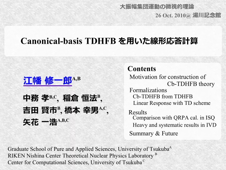
SLIDE 1 Canonical-basis TDHFB を用いた線形応答計算
大振幅集団運動の微視的理論 26 Oct. 2010@ 湯川記念館
江幡 修一郎A,B
中務 孝B,C, 稲倉 恒法B, 吉田 賢市B, 橋本 幸男A,C, 矢花 一浩A,B,C
Graduate School of Pure and Applied Sciences, University of TsukubaA RIKEN Nishina Center Theoretical Nuclear Physics Laboratory B Center for Computational Sciences, University of Tsukuba C
Contents
Formalizations Results
Comparison with QRPA cal. in ISQ
Motivation for construction of Cb-TDHFB theory
Cb-TDHFB from TDHFB Linear Response with TD scheme
Summary & Future
Heavy and systematic results in IVD
SLIDE 2
Propaganda of Phys. Rev. C82, 034306
SLIDE 3 from http://release.nikkei.co.jp/
Nikkei press release
from http://release.nikkei.co.jp/
RIKEN press release
SLIDE 4 from http://unedf.org/
Density Functional Theory
Introduction
SLIDE 5 from http://unedf.org/
Density Functional Theory
Introduction
W.J.Swiatecki, Phys. Rev. 100 (1955) 937
Spontaneous Fission Half-lives
J.L.Wood et.al, Phys. Rep. 215 (1992) 101
Gap Energy
2+ 0+
First 2+ state
50Sn Isotopes
From J.H.E.Mattauch, W.Thiele and A.H.Wapstra,
Odd-even mass staggering
SLIDE 6 from http://www.rarf.riken.go.jp/newcontents/contents/facility/RIBF.html
Introduction
SLIDE 7 from http://www.rarf.riken.go.jp/newcontents/contents/facility/RIBF.html
Introduction
Future plan of RI facility in the world
SLIDE 8
1, Applicable to heavy nuclei
Construction of theoretical framework to calculate structure and response of from light nuclei to heavy ones systematically
Cb-TDHFB
Requirements :
3-Dimensional coordinate-space
2, No symmetry restriction for any deformed nuclei 3, Able to describe excitations and various dynamics of nuclei 4, Including effects of Pairing Correlation
+
Introduction
SLIDE 9 TDHFB
Recipe for the Canonical-basis TDHFB (Cb-TDHFB)
: Density matrix : Pair tensor : Arbitrary complete set : Canonical basis Canonical-basis diagonalize Density matrix. In this Canonical-basis, the number of matrix elements compress to diagonal components. : Time-dependent Canonical basis
Ebata et al, PRC82, 034306
The computational cost of TDHFB may be reduced also in Canonical-basis representation !!
: Time-dependent Canonical single-particle basis This set is assumed to be orthonormal.
SLIDE 10 TDHFB
1, Canonical-basis representation
: Occupation probability : Pair probability : Normal density : Pair tensor
Recipe for the Cb-TDHFB
Ebata et al, PRC82, 034306 : Pair of k-state (no restriction of time-reversal)
Inversion We can get the derivatives of ρk(t) and κk(t) with respect to time.
SLIDE 11 Recipe for the Cb-TDHFB
Ebata et al, PRC82, 034306
TDHFB
We can get the time-dependent equation for with orthonormal canonical basis
?
ρk(t) and κk(t)
are identical to gap parameters of BCS approximations, in the case where pair potential is computed as
SLIDE 12 Recipe for the Cb-TDHFB
Ebata et al, PRC82, 034306
Can we describe the inversion for this part with the orthonormal canonical basis ?
2, Assumption for Pairing potential
… Pair potential is diagonal. We can not invert this pairing potential, because the two-particle state do not span the whole space.
We can invert the pairing potential.
Cb-TDHFB equations
Properties of Cb-TDHFB
TDHF HF+BCS
SLIDE 13 3, We adopt a schematic pairing functional:
Recipe for the Cb-TDHFB
Ebata et al, PRC82, 034306
This pairing potential violate the gauge invariance related to the phase degree of freedom of canonical basis.
Cb-TDHFB equations are invariant with respect to the phase of canonical basis.
This schematic pairing potential violate
We must choose the special gauge in this schematic pairing functional.
SLIDE 14 TDHFB
1, Canonical-basis representation 2, Assumption for Pairing potential
3, We adopt a schematic pairing functional. We must choose the special gauge.
Cb-TDHFB
Recipe for the Cb-TDHFB
Feasible Cb-TDHFB
Ebata et al, PRC82, 034306
SLIDE 15 Strength function S(E;F)
^
Instantaneous external field then the equations can be automaticaly linearised with respect to Vext and the density fluctuation.
Initial state of Real-Time cal. Ground state of HF or HF+BCS
Strength function is calculated as Fourier transformed time dependent expectation value of F.
^
How to calculate Linear Response with TD scheme ?
SLIDE 16 Interaction : Skyrme force (SkM*)
Even-even Nuclei : 18-32Ne, 18-40Mg, 24-46Si, 28-50S, 32-58Ar, 144-154Sm, 172Yb (12-22C, 14-28O, 34-64Ca) External field : Isovector Dipole, Isoscalar Quadrupole
- Cal. space (3D-Spherical box):
Calculation setup
Pairing strength : Smoothed Pairing strength
Pairing model space
Energy cutoff we use the box has radius 12 [fm] & mesh 0.8 [fm].
Relatively light nuclei case (A < 60), Relatively heavy nuclei case (A > 100),
we use the box has radius 15 [fm] & mesh 1.0 [fm].
SLIDE 17 Can we describe deformed nuclei ? in Quadrupole mode
16O 24Mg
β =0.00
∆n = 0.0 [MeV] ∆p = 0.0 [MeV] ∆n = 0.0 [MeV] ∆p = 0.0 [MeV]
β =0.39
In Spherical case, we can not distinguish Q20 and Q22 mode. In Quadrupole deformed case(prolate), the GR of Q20 is lower than one of Q22. K=0- K=1- In Spherical case, In oblate case, the relation between Q20 and Q22 is reversed.
SLIDE 18 Comparison with QRPA (IS Quadrupole) for 34Mg
34Mg
(a) Cb-TDHFB with fixed LS & Coulomb potentials (b) Full Cb-TDHFB (d) QRPA (delta-pairing)
- C. Losa et al.PRC81, 064307 (2010)
(c) QRPA without residual LS & Coulomb interaction (delta-pairing)
SLIDE 19 Summary of isoscalar Quadrupole mode
The results of Cb-TDHFB well agree with other deformed QRPA cal. in isoscalar quadrupole modes, except for height of the lowest peak.
( caused by using a schematic pairing functional ? )
The results of ISQ vibration are more sensitive for the residual spin-
- rbit interaction than ones of IVD mode.
In spherical case, we can not distinguish ISQ vibrations which are called β - and γ - vibration. In prolate (oblate) deformed case, main peak of Q20 is lower (higher) than one of Q22.
Comparison with deformed HFB+QRPA results for 34Mg and ///////
24 ////Mg
////// We can describe the properties of deformed nuclei for ISQ vibrations with Cb-TDHFB in 3D-coordinate space.
SLIDE 20 16O 24Mg
From J,IZV,67,656,2003
β =0.00
∆n = 0.0 [MeV] ∆p = 0.0 [MeV] ∆n = 0.0 [MeV] ∆p = 0.0 [MeV]
β =0.39
In Spherical case, the Giant Dipole Resonance(GDR) will be a concentrated peak. In Quadrupole deformed case, the GDR have two components, K=0-, 1- K=0- K=1-
Can we describe deformed nuclei ? in E1 mode
From Nucl.Phys. A251,479(1975)
SLIDE 21 Example of E1 mode for other heavier nuclei with SkM*
40Ca
∆n = 0.0 [MeV] ∆p = 0.0 [MeV]
β =0.00
90Zr
∆n = 0.0 [MeV] ∆p = 1.9 [MeV]
β =0.00
From Nucl.Phys. A175, 609 (1971) From Nucl.Phys. A227, 513 (1974)
208Pb
∆n = 0.0 [MeV] ∆p = 0.0 [MeV]
β =0.00
From Nucl.Phys. A159, 561 (1970)
SLIDE 22 ∆n = 0.9 [MeV] ∆p = 1.9 [MeV]
The shape transitional region in Sm isotopes
From Nucl.Phys. A225, 171 (1974)
β =0.00 β =0.00 β =0.11 β =0.32 β =0.29 β =0.20
Preliminary
N = 82 N = 84 N = 86
Preliminary
N = 88 N = 90
∆n = 0.0 [MeV] ∆p = 2.0 [MeV] ∆n = 0.9 [MeV] ∆p = 1.6 [MeV] ∆n = 0.9 [MeV] ∆p = 1.5 [MeV] ∆n = 1.0 [MeV] ∆p = 1.1 [MeV] ∆n = 0.9 [MeV] ∆p = 1.0 [MeV]
SLIDE 23 E1 strength functions 172Yb (for computational cost)
172Yb
PRC82, 034326
β =0.34
∆n = 0.773 [MeV] ∆p = 1.248 [MeV]
172Yb
β =0.32
∆n = 0.757 [MeV] ∆p = 0.551 [MeV]
( based on PRC82, 034306 ) Box size : R=15[fm], mesh=1[fm] (3D-Spherical) Box Size : ρ = z±=20[fm], b-spline (Cylindrical) Single-quasiparticle space (g.s. HFB) : 5348 states for neutron, 4648 states for proton Canonical basis space (g.s. HF+BCS) : 146 states for neutron, 98 states for proton Total time : 136,000 CPU hours (with Kraken; Super computer of ORNL) Total time : 300 CPU hours (with ONE CPU; Intel Core i7 3.0 GHz)
SLIDE 24 E1 strength functions for Ne isotopes
SLIDE 25 E1 strength functions for Mg isotopes
SLIDE 26
In order to investigate the appearance of Low-energy E1 strength ...
SLIDE 27 The ratio of the E1 strength in Low-energy region
Low-energy region < 10 [MeV] For Ne, Mg isotopes
The low-energy E1 strength appear from N=16 in the both cases. (They start to occupy the s1/2 orbit.) Spherical Deformed 16
SLIDE 28 The ratio of the E1 strength in Low-energy region
Low-energy region < 10 [MeV] For Si, S, Ar isotopes
The low-energy E1 strength appear dramatically from N=30 in the HF+RPA case. (They start to occupy the p3/2 orbit.) 30
SLIDE 29 Pygmy resonance is pure soft-dipole mode ?
SLIDE 30 Pygmy resonance is pure soft-dipole mode ?
24O 26O 26Ne 28Ne
N = 16 N = 16 N = 18 N = 18
SLIDE 31 Summary
Derivation of Cb-TDHFB from TDHFB with a simple assumption Linear Response calculations (for C,O,Ne,Mg,Si,S,Ar,Ca,Sm,Yb) for ISQ and IVD mode systematically using Cb-TDHFB
Comparison with HF+RPA results for Ne, Mg, Si, S, Ar isotopes The low-energy E1 strength is sensitive to low-momentum orbits and nuclear deformation. The Pairing correlation should be include to describe the occupation of these orbits. The appearance of the low-energy E1 strength of nearly magic number is smoothed by the continuous occupation of orbitals caused Pairing correlation. Comparison with deformed HFB+QRPA results for 172Yb Cb-TDHFB significantly reduces the computational cost.
For the E1 strength function of 172Yb: 136,000 → 300 CPU hours
Comparison with unperturbed results for N=16, 18 isotopes of O and Ne These results indicate that Pygmy resonance has not only collective part which likes soft-dipole mode, but also single-particle excitation.
SLIDE 32
Comparison with deformed HFB+QRPA results for 34Mg, 172Yb Comparison with HF+RPA results for Ne, Mg, Si, S, Ar isotopes
Derivation of Cb-TDHFB from TDHFB with a simple assumption
Summary
Application of Cb-TDHFB to systematic calculation with other modes(ISQ, ISO, IVM, etc.)
Future work
Application of Cb-TDHFB to heavy-ion collision
Linear Response calculations (for C,O,Ne,Mg,Si,S,Ar,Ca, Sm,Yb) for ISQ and IVD mode systematically using Cb-TDHFB
Comparison with unperturbed results for N=16, 18 isotopes of O and Ne
SLIDE 33 Energy cutoff function Smoothed Pairing
Gap equation Particle number equation
[ N.Tajima, et al. NPA603(1996)23]
SLIDE 34
: phase of
How to calculate time development ?