7 Neural MT 1: Neural Encoder-Decoder Models From Section 3 to - - PDF document

7 Neural MT 1: Neural Encoder-Decoder Models

From Section 3 to Section 6, we focused on the language modeling problem of calculating the probability P(E) of a sequence E. In this section, we return to the statistical machine translation problem (mentioned in Section 2) of modeling the probability P(E | F) of the

• utput E given the input F.

7.1 Encoder-decoder Models

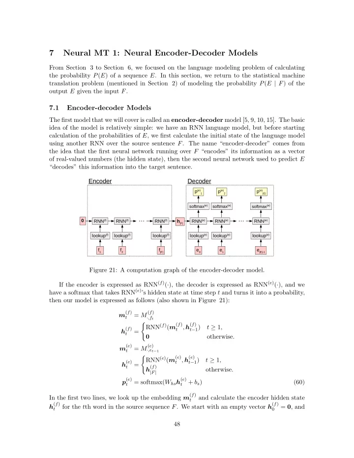
The first model that we will cover is called an encoder-decoder model [5, 9, 10, 15]. The basic idea of the model is relatively simple: we have an RNN language model, but before starting calculation of the probabilities of E, we first calculate the initial state of the language model using another RNN over the source sentence F. The name “encoder-decoder” comes from the idea that the first neural network running over F “encodes” its information as a vector

• f real-valued numbers (the hidden state), then the second neural network used to predict E

“decodes” this information into the target sentence.

f1 RNN(f) lookup(f) f2 RNN(f) lookup(f) f|F| RNN(f) lookup(f)

…

e0 RNN(e) lookup(e) e1 RNN(e) lookup(e) e|E|-1 RNN(e) lookup(e)

…

p(e)

1

p(e)

2

p(e)

|E|

softmax(e) softmax(e) softmax(e)

h|F|

Encoder Decoder Figure 21: A computation graph of the encoder-decoder model. If the encoder is expressed as RNN(f)(·), the decoder is expressed as RNN(e)(·), and we have a softmax that takes RNN(e)’s hidden state at time step t and turns it into a probability, then our model is expressed as follows (also shown in Figure 21): m(f)

t

= M(f)

·,ft

h(f)

t

= ( RNN(f)(m(f)

t

, h(f)

t−1)

t 1,

• therwise.

m(e)

t

= M(e)

·,et−1

h(e)

t

= ( RNN(e)(m(e)

t , h(e) t−1)

t 1, h(f)

|F|

• therwise.

p(e)

t

= softmax(Whsh(e)

t

+ bs) (60) In the first two lines, we look up the embedding m(f)

t

and calculate the encoder hidden state h(f)

t

for the tth word in the source sequence F. We start with an empty vector h(f) = 0, and 48

by h(f)

|F|, the encoder has seen all the words in the source sentence. Thus, this hidden state

should theoretically be able to encode all of the information in the source sentence. In the decoder phase, we predict the probability of word et at each time step. First, we similarly look up m(e)

t , but this time use the previous word et−1, as we must condition the

probability of et on the previous word, not on itself. Then, we run the decoder to calculate h(e)

t . This is very similar to the encoder step, with the important difference that h(e)

is set to the final state of the encoder h(f)

|F|, allowing us to condition on F. Finally, we calculate the

probability p(e)

t

by using a softmax on the hidden state h(e)

t .

While this model is quite simple (only 5 lines of equations), it gives us a straightforward and powerful way to model P(E | F). In fact, [15] have shown that a model that follows this basic pattern is able to perform translation with similar accuracy to heavily engineered systems specialized to the machine translation task (although it requires a few tricks over the simple encoder-decoder that we’ll discuss in later sections: beam search (Section 7.2), a different encoder (Section 7.3), and ensembling (??)).

7.2 Generating Output

At this point, we have only mentioned how to create a probability model P(E | F) and haven’t yet covered how to actually generate translations from it, which we will now cover in the next

• section. In general, when we generate output we can do so according to several criteria:

Random Sampling: Randomly select an output E from the probability distribution P(E | F). This is usually denoted ˆ E ⇠ P(E | F). 1-best Search: Find the E that maximizes P(E | F), denoted ˆ E = argmax

E

P(E | F). n-best Search: Find the n outputs with the highest probabilities according to P(E | F). Which of these methods we will choose will depend on our application, so we will discuss some use cases along with the algorithms themselves. 7.2.1 Random Sampling First, random sampling is useful in cases where we may want to get a variety of outputs for a particular input. One example of a situation where this is useful would be in a sequence- to-sequence model for a dialog system, where we would prefer the system to not always give the same response to a particular user input to prevent monotony. Luckily, in models like the encoder-decoder above, it is simple to exactly generate samples from the distribution P(E | F) using a method called ancestral sampling. Ancestral sampling works by sampling variable values one at a time, gradually conditioning on more context, so at time step t, we will sample a word from the distribution P(et | ˆ et−1

1

). In the encoder-decoder model, this means we simply have to calculate pt according to the previously sampled inputs, leading to the simple generation algorithm in Algorithm 3. One thing to note is that sometimes we also want to know the probability of the sentence that we sampled. For example, given a sentence ˆ E generated by the model, we might want to know how certain the model is in its prediction. During the sampling process, we can calculate P( ˆ E | F) = Q| ˆ

E| t

P(ˆ et | F, ˆ Et−1

1

) incrementally by stepping along and multiplying together 49

the probabilities of each sampled word. However, as we remember from the discussion of probability vs. log probability in Section 3.3, using probabilities as-is can result in very small numbers that cause numerical precision problems on computers. Thus, when calculating the full-sentence probability it is more common to instead add together log probabilities for each word, which avoids this problem. Algorithm 3 Generating random samples from a neural encoder-decoder

1: procedure Sample 2:

for t from 1 to |F| do

3:

Calculate m(f)

t

and h(f)

t

4:

end for

5:

Set ˆ e0 =“hsi” and t 0

6:

while ˆ et 6=“h/si” do

7:

t t + 1

8:

Calculate m(e)

t , h(e) t , and p(e) t

from ˆ et−1

9:

Sample ˆ et according to p(e)

t

10:

end while

11: end procedure

7.2.2 Greedy 1-best Search Next, let’s consider the problem of generating a 1-best result. This variety of generation is useful in machine translation, and most other applications where we simply want to output the translation that the model thought was best. The simplest way of doing so is greedy search, in which we simply calculate pt at every time step, select the word that gives us the highest probability, and use it as the next word in our sequence. In other words, this algorithm is exactly the same as Algorithm 3, with the exception that on Line 9, instead of sampling ˆ et randomly according to p(e)

t , we instead choose the max: ˆ

et = argmax

i

p(e)

t,i .

Interestingly, while ancestral sampling exactly samples outputs from the distribution ac- cording to P(E | F), greedy search is not guaranteed to find the translation with the highest

• probability. An example of a case in which this is true can be found in the graph in Fig-

ure 22, which is an example of search graph with a vocabulary of {a, b, h/si}.28 As an exercise, I encourage readers to find the true 1-best (or n-best) sentence according to the probability P(E | F) and the probability of the sentence found according to greedy search and confirm that these are different. 7.2.3 Beam Search One way to solve this problem is through the use of beam search. Beam search is similar to greedy search, but instead of considering only the one best hypothesis, we consider b best hypotheses at each time step, where b is the “width” of the beam. An example of beam search where b = 2 is shown in Figure 23 (note that we are using log probabilities here because they

28In reality, we will never have a probability of exactly P(et = h/si | F, et−1 1

) = 1.0, but for illustrative purposes, we show this here.

50

e1 P(e1|F)

<s> “a” “b” </s> “a” “b” </s> “a” “b” </s> </s> </s> </s> </s>

e2 P(e2|F,e1) e3 P(e3|F,e1,e2) e0 0.35 0.4 0.25 0.15 0.8 0.1 0.5 0.4 1.0 1.0 0.05 1.0 1.0

Figure 22: A search graph where greedy search fails.

log P(e1|F)

<s> “a” “b” </s> “a” “b” </s> “a” “b” </s> </s> </s>

log P(e2|F,e1) log P(e3|F,e1,e2)

• 1.05
• 0.92
• 1.39
• 1.90
• 0.22
• 2.30
• 0.69
• 0.92
• 3.00
• 1.05
• 0.92
• 1.39

X

• 2.95
• 1.27
• 4.05
• 1.84
• 1.61
• 3.22

X X X X

• 1.27
• 1.61

Figure 23: An example of beam search with b = 2. Numbers next to arrows are log probabil- ities for a single word log P(et | F, et−1

1

), while numbers above nodes are log probabilities for the entire hypothesis up until this point. 51

are more conducive to comparing hypotheses over the entire sentence, as mentioned before). In the first time step, we expand hypotheses for e1 corresponding to all of the three words in the vocabulary, then keep the top two (“b” and “a”) and delete the remaining one (“h/si”). In the second time step, we expand hypotheses for e2 corresponding to the continuation of the first hypotheses for all words in the vocabulary, temporarily creating b⇤|V | active hypotheses. These active hypotheses are also pruned down to the b active hypotheses (“a b” and “b b”). This process of calculating scores for b ⇤ |V | continuations of active hypotheses, then pruning back down to the top b, is continued until the end of the sentence. 7.2.4 Length Normalization One thing to be careful about when generating sentences using models, such as neural ma- chine translation, where P(E | F) = Q|E|

t

P(et | F, et−1

1

) is that they tend to prefer shorter

• sentences. This is because every time we add another word, we multiply in another probabil-

ity, reducing the probability of the whole sentence. As we increase the beam size, the search algorithm gets better at finding these short sentences, and as a result, beam search with a larger beam size often has a significant length bias towards these shorter sentences. There have been several attempts to fix this length bias problem. For example, it is possible to put a prior probability on the length of the sentence given the length of the source sentence P(|E| | |F|), and multiply this with the standard sentence probability P(E | F) at decoding time [8]: ˆ E = argmax

E

log P(|E| | |F|) + log P(E | F). (61) This prior probability can be estimated from data, and [8] simply estimate this using a multinomial distribution learned on the training data: P(|E| | |F|) = c(|E|, |F|) c(|F|) . (62) A more heuristic but still widely used approach normalizes the log probability by the length

• f the target sentence, effectively searching for the sentence that has the highest average log

probability per word [4]: ˆ E = argmax

E

log P(E | F)/|E|. (63)

7.3 Bidirectional Encoders

In Section 7.1, we described a model that works by encoding sequences linearly, one word at a time from left to right. However, this may not be the most natural or effective way to turn the sentence F into a vector h. The first solution to this problem is due to [15], the reverse encoder. In this method, we simply run a standard linear encoder over F, but instead of doing so from left to right, we do so from right to left.

• h (f)

t

= (

• RNN(f)(m(f)

t

,

• h (f)

t+1)

t  |F|,

• therwise.

(64) The motivation behind this method is that for pairs of languages with similar ordering (such as English-French, which the authors experimented on), the words at the beginning of F will 52

f1 enc f2 enc

… (a) Dependency Distances in Forward Encoder

enc f|F| e0 dec e1 e1 dec e2

…

enc e|E| e|E|-1

|F| |F| |F|

f|F| enc f|F|-1 enc

…

enc f1 e0 dec e1 e1 dec e2

…

enc e|E| e|E|-1

3 1 |F|+|E|-1 (b) Dependency Distances in Reverse Encoder

Figure 24: The distances between words with the same index in the forward and reverse decoders. generally correspond to words at the beginning of E. Assuming the extreme case that words with identical indices correspond to each-other (e.g. f1 corresponds to e1, f2 to e2, etc.), the distance between corresponding words in the linear encoding and decoding will be |F|, as shown in Figure 24(a). Remembering the vanishing gradient problem from Section 6.3, this means that the RNN has to propagate the information across |F| time steps before making a prediction, a difficult feat. At the beginning of training, even RNN variants such as LSTMs have trouble, as they have to essentially “guess” what part of the information encoded in their hidden state is being used without any prior bias. Reversing the encoder helps solve this problem by reducing the length of dependencies for a subset of the words in the sentence, specifically the ones at the beginning of the sentences. As shown in Figure 24(b), the length of the dependency for f1 and e1 is 1, and subsequent pairs of ft and et have a distance of 2t1. During learning, the model can “latch on” to these short-distance dependencies and use them as a way to bootstrap the model training, after which it becomes possible to gradually learn the longer dependencies for the words at the end

• f the sentence. In [15], this proved critical to learn effective models in the encoder-decoder

framework. However, this approach of reversing the encoder relies on the strong assumption that the

• rder of words in the input and output sequences are very similar, or at least that the words

at the beginning of sentences are the same. This is true for languages like English and French, which share the same “subject-verb-object (SVO)” word ordering, but may not be true for more typologically distinct languages. One type of encoder that is slightly more robust to these differences is the bi-directional encoder [2]. In this method, we use two different 53

encoders: one traveling forward and one traveling backward over the input sentence

• !

h (f)

t

= (

• !

RNN(f)(m(f)

t

, ! h (f)

t+−)

t 1,

• therwise.

(65)

• h (f)

t

= (

• RNN(f)(m(f)

t

,

• h (f)

t+1)

t  |F|,

• therwise.

(66) which are then combined into the initial vector h(e) for the decoder RNN. This combination can be done by simply concatenating the two final vectors ! h |F| and

• h 1. However, this also

requires that the size of the vectors for the decoder RNN be exactly equal to the combined size of the two encoder RNNs. As a more flexible alternative, we can add an additional parameterized hidden layer between the encoder and decoder states, which allows us to convert the bidirectional encoder states into an appropriately-sized state for the decoder: h(e) = tanh(W−

→ f e

• !

h |F| + W←

− f e

• h 1 + be).

(67)

7.4 Sentence Embedding Methods

One interesting feature of the encoder-decoder model is that it compresses an entire input sentence F to a single vector h(f)

|F|. Having a mapping function of this variety can be useful

in other downstream tasks. For example, in text classification, we can use the encoder to

• btain the hidden vector h(f)

|F|, then run this vector itself through a classifier to predict some

• ther feature of the text, such as topic or sentiment.

An advantage of this paradigm is that translation data is relatively easy to come by compared to data manually labeled with sentiment or topic labels, and thus a translation system can be used to pre-train the encoder for use in this downstream task. In addition, it is common to train these models using other varieties of data as well: Auto-encoding: The parameters are trained on a plain text corpus, where the encoder encodes a sentence into a single vector, and the decoder tries to re-generate the sentence itself [7]. Language modeling: Similarly, the parameters are trained on a plain text corpus, where after each time step in the encoder tries to predict the word using the previously- described RNN language models. This is used as a pre-training step, and the model can then be fine-tuned on the actual task (such as text classification) [7]. This variety of language-model-based pre-training has proven an effective way to improve translation systems as well [14]. Predicting context: Parameters are trained on a corpus of documents, where the encoder encodes a sentence, and two decoders try to predict the previous and next sentences [11]. Predicting paraphrases: Parameters are trained on a corpus of paraphrases, where the encoder is trained to make the vectors of paraphrases closer together than the vectors

• f non-paraphrases [16].

54

Predicting sentence features: Parameters are trained on data with supervised labels of some variety, such as entailment relations between multiple sentences [6]. These methods are a specific variety of multi-task learning, where we use training data for

• ne task to improve accuracy on another, which will be covered more extensively in Section 21.

7.5 Further Reading

First, a brief historical note on neural machine translation models. [1] first proposed the idea of performing translation using neural networks, with a simple feed-forward model that mapped between short sentences. [5] further expanded this to recurrent networks, which more closely represent those that proved successful in [15]’s experiments. The first example of fully neural models for translation in the modern era of deep learning is due to [10], which used convolutional networks, to be covered in the following chapters. This was followed shortly thereafter by [15], which popularized neural MT due to impressive empirical performance, which can be largely attributed to the switch from RNNs to deep LSTMs, reverse encoder, use of beam search and ensembling, etc. In addition, in this chapter, we illustrated in particular detail search algorithms such as beam search. Beam search based methods can further be improved with the introduction of a future cost, which predicts how likely particular search paths are to succeed [12]. It is also possible to start from a greedy search, then gradually expand search paths that look most promising [3].

7.6 Exercise

In the exercise for this chapter, we will create an encoder-decoder translation model and make it possible to generate translations. Writing the program will entail:

• Extend your RNN language model code to first read in a source sentence to calculate

the initial hidden state.

• On the training set, write code to calculate the loss function and perform training.
• On the development set, generate translations using greedy search.
• Evaluate your generated translations by comparing them to the reference translations

to see if they look good or not. Translations can also be evaluated by automatic means, such as BLEU score [13]. A reference implementation of a BLEU evaluation script can be found here: https://github.com/moses-smt/mosesdecoder/blob/master/scripts/ generic/multi-bleu.perl. Potential improvements to the model include: Implementing beam search and comparing the results with greedy search. Implementing an alternative encoder.

References

[1] Robert B Allen. Several studies on natural language and back-propagation. In Proceedings of the IEEE First International Conference on Neural Networks, volume 2, page 341. IEEE Piscataway, NJ, 1987.

55

[2] Dzmitry Bahdanau, Kyunghyun Cho, and Yoshua Bengio. Neural machine translation by jointly learning to align and translate. In Proceedings of the International Conference on Learning Rep- resentations (ICLR), 2015. [3] Jacob Buckman, Miguel Ballesteros, and Chris Dyer. Transition-based dependency parsing with heuristic backtracking. In Proceedings of the 2016 Conference on Empirical Methods in Natural Language Processing (EMNLP), pages 2313–2318, 2016. [4] Kyunghyun Cho, Bart van Merrienboer, Dzmitry Bahdanau, and Yoshua Bengio. On the proper- ties of neural machine translation: Encoder–decoder approaches. In Proceedings of the Workshop

• n Syntax and Structure in Statistical Translation, pages 103–111, 2014.

[5] Lonnie Chrisman. Learning recursive distributed representations for holistic computation. Con- nection Science, 3(4):345–366, 1991. [6] Alexis Conneau, Douwe Kiela, Holger Schwenk, Lo¨ ıc Barrault, and Antoine Bordes. Supervised learning of universal sentence representations from natural language inference data. In Proceedings

• f the 2017 Conference on Empirical Methods in Natural Language Processing (EMNLP), pages

670–680, 2017. [7] Andrew M Dai and Quoc V Le. Semi-supervised sequence learning. In Proceedings of the 29th Annual Conference on Neural Information Processing Systems (NIPS), pages 3079–3087, 2015. [8] Akiko Eriguchi, Kazuma Hashimoto, and Yoshimasa Tsuruoka. Tree-to-sequence attentional neu- ral machine translation. In Proceedings of the 54th Annual Meeting of the Association for Com- putational Linguistics (ACL), pages 823–833, 2016. [9] Mikel L Forcada and Ram´

• n P ˜
• Neco. Recursive hetero-associative memories for translation. In

International Work-Conference on Artificial Neural Networks, pages 453–462. Springer, 1997. [10] Nal Kalchbrenner and Phil Blunsom. Recurrent continuous translation models. In Proceedings

• f the 2013 Conference on Empirical Methods in Natural Language Processing (EMNLP), pages

1700–1709, 2013. [11] Ryan Kiros, Yukun Zhu, Ruslan R Salakhutdinov, Richard Zemel, Raquel Urtasun, Antonio Torralba, and Sanja Fidler. Skip-thought vectors. In Proceedings of the 29th Annual Conference

• n Neural Information Processing Systems (NIPS), pages 3294–3302, 2015.

[12] Jiwei Li, Will Monroe, and Dan Jurafsky. Learning to decode for future success. arXiv preprint arXiv:1701.06549, 2017. [13] Kishore Papineni, Salim Roukos, Todd Ward, and Wei-Jing Zhu. BLEU: a method for automatic evaluation of machine translation. In Proceedings of the 40th Annual Meeting of the Association for Computational Linguistics (ACL), pages 311–318, 2002. [14] Prajit Ramachandran, Peter Liu, and Quoc Le. Unsupervised pretraining for sequence to sequence learning. In Proceedings of the 2017 Conference on Empirical Methods in Natural Language Processing (EMNLP), pages 383–391, 2017. [15] Ilya Sutskever, Oriol Vinyals, and Quoc VV Le. Sequence to sequence learning with neural

• networks. In Proceedings of the 28th Annual Conference on Neural Information Processing Systems

(NIPS), pages 3104–3112, 2014. [16] John Wieting, Mohit Bansal, Kevin Gimpel, and Karen Livescu. Towards universal paraphrastic sentence embeddings. Proceedings of the International Conference on Learning Representations (ICLR), 2015.

56