SLIDE 43 43/63
<Go>
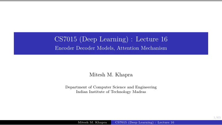
1 I am 1 am going 1 going home 1 home <STOP> 1 x1 Main i/p: x2 ghar x3 ja x4 raha x5 hoon hi + c3 α1,3 α2,3 α3,3 α4,3 α5,3 + c2 α1,2 α2,2α3,2α4,2 α5,2 + α1,4α2,4α3,4 α4,4 α5,4 c4 + α1,5 α2,5α3,5α4,5 α5,5 c5
Task: Machine Translation Data: {xi = sourcei, yi = targeti}N
i=1
Encoder: ht = RNN(ht−1, xt) s0 = hT Decoder: ejt = VT
attntanh(Uattnhj + Wattnst)
αjt = softmax(ejt) ct =
T
∑
j=1
αjthj st = RNN(st−1, [e(ˆ yt−1), ct]) ℓt = softmax(Vst + b) Parameters: Udec, V, Wdec, Uenc, Wenc, b, Uattn, Vattn Loss and Algorithm remains same
Mitesh M. Khapra CS7015 (Deep Learning) : Lecture 16