7. Entropy as a Thermodynamic Variable S 1 gives us T E d T /W =0 - - PowerPoint PPT Presentation

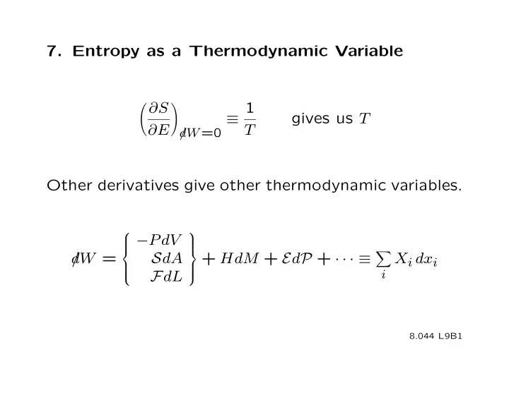
• 7. Entropy as a Thermodynamic Variable

∂S 1 ≡ gives us T ∂E d

/W =0

T Other derivatives give other thermodynamic variables.

⎧ ⎪ ⎪ ⎨ ⎫ ⎪ ⎪ ⎬

−P dV SdA d /W = + HdM + EdP + · · · ≡ Xi dxi

⎪ ⎪ ⎩ ⎪ ⎪ ⎭

i

FdL

8.044 L9B1

We chose to use the extensive external variables (a complete set) as the constraints on Ω. Thus S ≡ k ln Ω = S( E, V, M, · · · ) Now solve for E. S(E, V, M, · · ·) ↔ E(S, V, M, · · ·) We know dE|d = d /Q from the 1ST law

/W =0

dE|d

/W =0 ≤ T dS

utilizing the 2ND law

8.044 L9B2

Now include the work. dE = d /Q + d /W dE ≤ T dS + d /W

    −P dV

SdA

   

dE ≤ T dS + + HdM + EdP + · · ·

  

FdL

  

The last line expresses the combined 1ST and 2ND laws of thermodynamics.

8.044 L9B3

Solve for dS. 1 P H E dS = dE + dV − dM − dP + · · · T T T T Examine the partial derivatives of S.

∂S

= 1

∂S

= − H ∂E

V,M,P

T ∂M

E,V,P

T

∂S

= P

⎛ ⎝ ∂S ⎞ ⎠

= − Xj ∂V

E,M,P

T ∂xj E,xi T

=xj

8.044 L9B4

INTERPRETATION

S(E,V) E V

dS =

∂S

∂E

• V

dE +

∂S

∂V

• E

dV = 1 T dE + P T dV

8.044 L9B5

UTILITY Internal Energy

 

∂S(E, V, N) 1

 

= → T (E, V, N) ↔ E(T, V, N) ∂E T

V

Equation of State

 

∂S(E, V, N) P

 

= → P (E, T, V, N) → P (T, V, N) ∂V T

E

8.044 L9B6

Example Ideal Gas

⎧ ⎪ ⎨ ⎫ ⎪ ⎬ 3/2

4 E S(E, N, V ) = k ln Φ = kN ln V πem 3 N

⎪ ⎩ ⎪ ⎭ ∂S

kN {} kN P = = = ∂V

E,N

{} V V T PV = NkT

8.044 L9B7

COMBINATORIAL FACTS # different orderings (permutations) of K distin- guishable objects = K! # of ways of choosing L from a set of K: K! if order matters (K − L)! K! if order does not matter L!(K − L)!

8.044 L9B8a

EXAMPLE Dinner Table, 5 Chairs (places) Seating, 5 people 5·4·3·2·1 = 5! = 120 Seating, 3 people 5 · 4 · 3 = 5! = 60

2! 1

Place settings, 3 people 5·4·3/6 = 5!

3! = 10 2!

8.044 L9B8b

• ε

> >

• ε

8.044 L9B9

• ε
• ε
• ε

8.044 L9B10

N!

1 when N1 = 0 or N Ω(E) = N1!(N−N1)! Maximum when N1 = N/2 S(E) = k ln Ω(E)

S(E) E T>0 T<0 T=0 T= (or - ) E = ε N E = ε N/2

8.044 L9B11

ln N! ≈ N ln N − N S(E) = k[N ln N − N1 ln N1 − (N − N1) ln(N − N1) − N + N1 + N − N1] 1 ∂S ∂S ∂N1 k = = = [−1 − ln N1 + 1 + ln(N − N1)] T ∂E

N

∂N1 ,∂E

af

E

1/E

⎛ ⎞ ⎛ ⎞

k N − N1 k N

⎝ ⎠ ⎝ ⎠

= ln = ln − 1 E N1 E N1

8.044 L9B12

N N

E/kT

− 1 = e → N1 = E/kT + 1 N1 e EN E = EN1 = E/kT + 1 e

kT/ε

1.0 0.5 1 2 3 4

N1/N or E/εN

−ε/kT

e

~ ~

8.044 L9B13

• 2

E/kT

∂E E e C ≡ = Nk ∂T kT (eE/kT + 1)2

• 2
• 2

E Nk E

−E/kT

→ Nk e low T , → high T kT 4 kT

1 2 3 4 0.1 0.2 0.3 0.4 0.5

kT/ε C/Nk

8.044 L9B14

p(n) =? n = 0, 1 In Ω' N → N − 1 and p(n) = Ω' Ω N1 → N1 − n p(n) =

(N−1)! (N1−n)!(N−1−N1+n)! N! N1!(N−N1)!

8.044 L9B15

• (N − 1)!

N1! (N − N1)! p(n) = N! (N1 − n)! (N − N1 − 1 + n)!

• 1/N

1 n = 0 N − N1 n = 0 N1 n = 1 1 n = 1

⎫

p(0) = N−N1 = 1 − N1

⎪ ⎪ ⎪

N N

⎬

p(0) + p(1) = 1

⎪ ⎪ ⎪

p(1) = N1 = [eE/kT + 1]−1

⎭

N

8.044 L9B16

1 2 3 4 0.5 1

p(0) p(1) kT/ε

p(n) n 1

EN E = (0)N p(0) + (E)N p(1) = E/kT + 1 e But we knew E, so we could have worked back- wards to find p(1).

8.044 L9B17

• Ω
• Ω/Ω
• 8.044 L9B18

The microcanonical ensemble is the starting point for Statistical Mechanics.

• We will no longer use it to solve problems.
• We will develop our understanding of the 2ND law.
• We will derive the canonical ensemble, the real

workhorse of S.M.

8.044 L9B19

MIT OpenCourseWare http://ocw.mit.edu

8.044 Statistical Physics I

Spring 2013 For information about citing these materials or our Terms of Use, visit: http://ocw.mit.edu/terms.