7 0 equality contraints lagrange multipliers
play

7.0 Equality Contraints: Lagrange Multipliers Consider the - PDF document

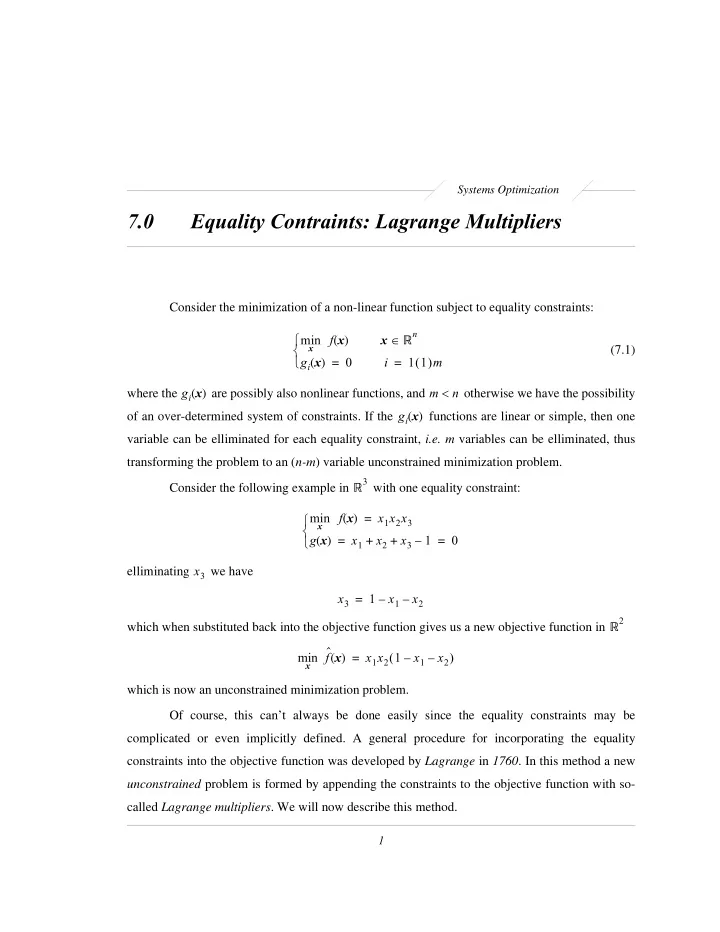
Systems Optimization 7.0 Equality Contraints: Lagrange Multipliers Consider the minimization of a non-linear function subject to equality constraints: R n min f x ( ) x (7.1) x ( ) m g i x ( ) = 0 i = 1 1 <


  1. Systems Optimization 7.0 Equality Contraints: Lagrange Multipliers Consider the minimization of a non-linear function subject to equality constraints: R n ∈ ⎧ min f x ( ) x (7.1) ⎨ x ( ) m ⎩ g i x ( ) = 0 i = 1 1 < where the g i x ( ) are possibly also nonlinear functions, and m n otherwise we have the possibility of an over-determined system of constraints. If the g i x ( ) functions are linear or simple, then one variable can be elliminated for each equality constraint, i.e. m variables can be elliminated, thus transforming the problem to an ( n-m ) variable unconstrained minimization problem. Consider the following example in R 3 with one equality constraint: ( ) = min f x x 1 x 2 x 3 ⎧ x ⎨ ( ) = + + – = g x x 1 x 2 x 3 1 0 ⎩ elliminating x 3 we have x 3 = 1 – x 1 – x 2 which when substituted back into the objective function gives us a new objective function in R 2 ˆ x ( ) min f ( ) = x 1 x 2 1 – x 1 – x 2 x which is now an unconstrained minimization problem. Of course, this can’t always be done easily since the equality constraints may be complicated or even implicitly defined. A general procedure for incorporating the equality constraints into the objective function was developed by Lagrange in 1760 . In this method a new unconstrained problem is formed by appending the constraints to the objective function with so- called Lagrange multipliers . We will now describe this method. 1

  2. Systems Optimization 7.1 Lagrange Multipliers If we have an objective function in R n with m equality constraints, such as in (7.1) then we can introduce m new variables called Lagrange multipliers , λ i , i ( ) m = 1 1 (7.2) to create a new objective function is called the Lagrangian , L x λ ( , ) , defined as m ∑ L x λ ( , ) λ i g i x = f x ( ) + ( ) . (7.3) i = 1 We now must minimize the Lagrangian over the R n + m space of the original variables x plus the new Lagrange multipliers λ . Therefore, we have elliminated the equality constraints at the expense of increasing the dimension of our problem from R n to R n + m . We can now apply the optimality conditions as before. Recall the first order necessary condition that the minimum be at a stationary point. Therefore, if we take the gradient of the Lagrangian function we arrive at the following necessary conditions: ⎧ m ⎪ ∂ g i x ( ) ∂ ∂ L f ∑ ⎪ λ i ( ) n - - - - - - - - - - - - - - - - - - - - - = - - - - - - - + = 0 j = 1 1 ∂ ∂ ∂ ⎪ x j x j x j ⎪ x ∗ i = 1 x = (7.4) ⎨ λ∗ λ = ⎪ ⎪ ∂ L ⎪ g i x ∗ ( ) m - - - - - - - = ( ) = 0 i = 1 1 ⎪ ∂ λ i ⎩ These simultaneous equations are solved for x ∗ λ∗ ( , ) , that is, we have m + n equations in m + n unknowns. Note that the second set of these equations are just the original constraints! Also, since at the stationary point of the Lagrangian, x ∗ λ∗ ( , ) , we have g i x ∗ ( ) = 0 this means that L x ∗ λ∗ f x ∗ ( , ) = ( ) (7.5) but it is not necessarily the case that ∇ f x ∗ ( ) = . That is, in a problem where we have equality 0 constraints, the minimum is not necessarily found at a stationary point of the original objective 2

  3. Equality Constraints Lagrange Multipliers function. If ∇ f x ∗ ( ) = 0 then is is because the feasible region defined by the equality constraints includes the unconstrained minimum of the function. The use of this method can be cleared up by considering an example. Consider the following simple problem in R 2 with one equality constraint: ⎧ 1 2 2 ( ) ( ) = - - - x 1 + ⎪ min f x x 2 2 x ⎨ ⎪ 2 x 1 – x 2 = 5 ⎩ Geometrically, the problem is to find the point of shortest distance from the origin x 2 2 x 1 – x 2 = 5 x 1 2 λ = – x 1 2 2 length = x 1 + x 2 λ x 2 = ∴ ∝ f x ( ) length Figure 7.1 Simple equality constrained example. Method 1: Ellimination of a variable The first method we try is to elliminate one of the variables. Therefore, solving for x 2 in terms of x 1 we have x 2 = 2 x 1 – 5 which when substituted back into the objective function, gives us a new objective function of just one variable 1 ˆ x 1 2 ) 2 ( ) - - x 1 ( ( ) f = + 2 x 1 – 5 2 ˆ ∂ f * * ( ) 2 - - - - - - - - = x 1 + 2 x 1 – 5 = 0 ∂ x 1 * x 1 3

  4. Systems Optimization * gives us x 1 * * ( , ) Solving for x 1 = 2 , x 2 = – 1 ; that is x * = 2 – 1 . This is a very simple example because the equality constraint was such that one of the decision variables could be easily elliminated. We will now see how the Lagangian method can be used to solve the same problem. Method 2 : Lagrangian We first construct the Lagrangian as 1 2 2 L x λ ( , ) ( ) λ 2 x 1 ( ) = - - x 1 - + x 2 + – x 2 – 5 2 and then set the gradient of this function to zero: ⎧ ∂ L ⎪ 2 λ * = x 1 * + = 0 ⎪ ∂ x 1 ⎪ ⎪ ∂ L λ * ⎨ = x 2 * – = 0 ∂ x 2 ⎪ ⎪ ⎪ ∂ L = 2 x 1 * – x 2 * – 5 = 0 ⎪ ∂ λ ⎩ This is a set of 3 equations in 3 unknowns. We first solve the first two for the Lagrange multiplier, λ * , and then substitute into the third, giving 4 λ * λ * λ * ⇒ – – – 5 = 0 = – 1 Once we have the Lagrange multiplier, we can easily solve for the remaining variables ( x *, λ * ) ( , , ) = 2 – 1 – 1 This Lagrangian, L , is a quadratic function which can be written in matrix form as x 1 x 1 1 0 2 1 - - x 1 x 2 λ - L = + – – 0 0 5 x 2 0 1 1 x 2 2 2 – 1 0 λ λ from which we see that the Hessian matrix is given by 1 0 2 = A 0 1 – 1 – 2 1 0 , A is not positive definite nor semi-definite. Therefore, the solution x *, λ * ( ) and since A = – 5 is not a minimum of L x λ ( , ) but x * is a minimum of the constrained function f x ( ) . We now 4

  5. Equality Constraints Lagrange Multipliers check A – to see if it is positive definite. Since – A = – 1 , A is not a negative definite nor negative semi-definite. Therefore the solution x *, λ * ( ) is a saddle point of the Lagrangian function. 7.2 Quadratic Objective Functions with Linear Equality Constraints We now consider the specialized problem wherein the objective function is a positive R n ∈ definite quadratic function in n variables, x , and there exist m linear equality constraints < given by the matrix equation C x = . For a solution to exist we must have m . Thus we have: d n 1 - x T A x b T x ( ) = - - + minimize f x 2 x subject to: C x = d where A is an nxn positive definite matrix, and C is an mxn matrix with rank C = m . The Lagrangian is easily formed as 1 λ T C x - x T A x b T x L x λ ( , ) - - [ ] = + + – d 2 where λ is a column vector of m Lagrange multipliers. The necessary conditions for an extremum are now written as: C T λ * ⎧ ∇ x L x *, λ * ( ) = A x * + b + = 0 ⎨ ∇ λ L x *, λ * ( ) ⎩ = – = C x * d 0 which are a system of n + m equations and n + m unknowns. These can be succinctly written as: A C T – x * b = λ * d C O ( ) × ( ) R n + m n + m ∈ If we define a new matrix M such that A C T M = C O then we can write the solution as 5

  6. Systems Optimization – x * b M 1 – = λ * d – exists, and the solution x *, λ * If M is nonsignular, then M 1 ( ) exists. Alternatively, we can develop a solution by first soving for x * in terms of λ * from the first set of equations. Therefore we have – b – C T λ * A 1 – C T λ * A 1 A 1 ( ) b ( ) x * = – + = – – and substituting this into the second set of equations – b – C T λ * A 1 A 1 ( ) – – = C d . This is easily solved for the Lagrange multipliers as – C T – b – 1 CA 1 CA 1 λ * ( ) ( ) = – d + . – b – C T λ * A 1 A 1 This is substituted back into the solution x * = – – which gives – b – C T – C T – b – 1 A 1 A 1 CA 1 CA 1 ( ( ) ( ) ) x * = – – – d + Example: As an example, consider the minimization of the linearly constrained positive definite quadratic function x 2 2 2 minimize f x ( ) = + x 2 + x 3 1 x + + = x 1 2 x 2 3 x 3 7 subject to: 9 2 x 1 + 2 x 2 + x 3 = - - - 2 In matrix notation, the objective function becomes 1 - x T I x - f x ( ) = 2 1 0 0 A = I = 0 1 0 0 0 1 and the constraints are written as 6

  7. Equality Constraints Lagrange Multipliers 7 1 2 3 C x = d C = d = 9 - - - 2 2 1 2 We can now form the Lagrangian as 1 λ T C x - x T x L x λ ( , ) [ ] = - + – d 2 with the necessary conditions for an extremum given by * x 1 0 1 0 0 1 2 * 0 x 2 0 1 0 2 2 I C T x * 0 = = * 0 0 1 3 1 x 3 λ * 7 C O 1 2 3 0 0 * λ 1 9 - - - 2 2 1 0 0 2 * λ 2 We could invert the matrix 1 0 0 1 2 0 1 0 2 2 I C T M = = 0 0 1 3 1 C O 1 2 3 0 0 2 2 1 0 0 T variables. On the other hand, we can proceed as we did in order to solve for the x * λ * previously by first solving for x * in terms of λ * from the first set of equations. Thus we have C T λ * x * + = 0 C T λ * x * = – which can be substituted into the second set of equations C T λ * ( ) C – = d This can be solved for λ * as – d 1 CC T λ * ( ) = – For our particular problem, we have 7

Download Presentation
Download Policy: The content available on the website is offered to you 'AS IS' for your personal information and use only. It cannot be commercialized, licensed, or distributed on other websites without prior consent from the author. To download a presentation, simply click this link. If you encounter any difficulties during the download process, it's possible that the publisher has removed the file from their server.

Recommend


More recommend