4 Language Models 2: Log-linear Language Models This chapter will - PDF document

4 Language Models 2: Log-linear Language Models This chapter will discuss another set of language models: log-linear language models [9, 4], which take a very di ff erent approach than the count-based n -grams described above. 11 4.1 Model Formulation Like n -gram language models, log-linear language models still calculate the probability of a particular word e t given a particular context e t � 1 t � n +1 . 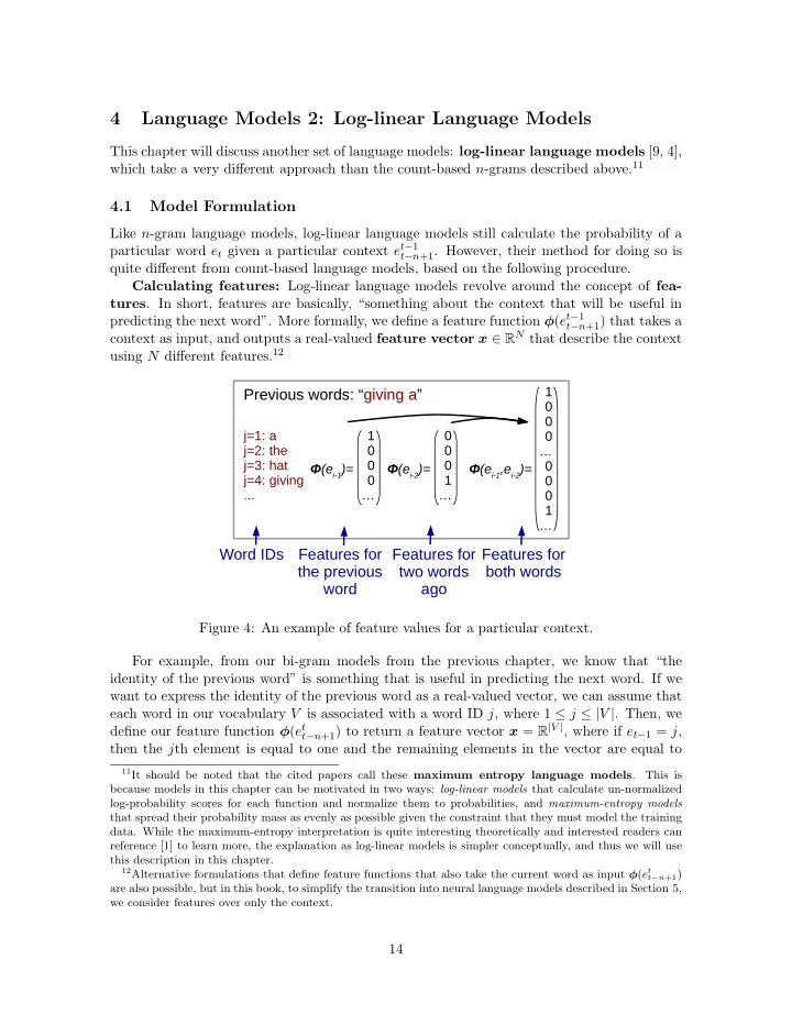However, their method for doing so is quite di ff erent from count-based language models, based on the following procedure. Calculating features: Log-linear language models revolve around the concept of fea- tures . In short, features are basically, “something about the context that will be useful in predicting the next word”. More formally, we define a feature function φ ( e t � 1 t � n +1 ) that takes a context as input, and outputs a real-valued feature vector x ∈ R N that describe the context using N di ff erent features. 12 1 Previous words: “giving a” 0 0 j=1: a 1 0 0 j=2: the 0 0 … j=3: hat 0 0 0 Φ (e i-1 )= Φ (e i-2 )= Φ (e i-1 ,e i-2 )= j=4: giving 0 1 0 ... … … 0 1 … Word IDs Features for Features for Features for the previous two words both words word ago Figure 4: An example of feature values for a particular context. For example, from our bi-gram models from the previous chapter, we know that “the identity of the previous word” is something that is useful in predicting the next word. If we want to express the identity of the previous word as a real-valued vector, we can assume that each word in our vocabulary V is associated with a word ID j , where 1 ≤ j ≤ | V | . Then, we define our feature function φ ( e t t � n +1 ) to return a feature vector x = R | V | , where if e t � 1 = j , then the j th element is equal to one and the remaining elements in the vector are equal to 11 It should be noted that the cited papers call these maximum entropy language models . This is because models in this chapter can be motivated in two ways: log-linear models that calculate un-normalized log-probability scores for each function and normalize them to probabilities, and maximum-entropy models that spread their probability mass as evenly as possible given the constraint that they must model the training data. While the maximum-entropy interpretation is quite interesting theoretically and interested readers can reference [1] to learn more, the explanation as log-linear models is simpler conceptually, and thus we will use this description in this chapter. 12 Alternative formulations that define feature functions that also take the current word as input φ ( e t t − n +1 ) are also possible, but in this book, to simplify the transition into neural language models described in Section 5, we consider features over only the context. 14

Previous words: “giving a” a 3.0 -6.0 -0.2 -3.2 the 2.5 -5.1 -0.3 -2.9 talk -0.2 0.2 1.0 1.0 b = w 1,a = w 2,giving = s = gift 0.1 0.1 2.0 2.2 hat 1.2 0.6 -1.2 0.6 … … … … … How likely How likely Words How likely Total given the given two we're are they? score previous words before predicting word is “a”? is “giving”? Figure 5: An example of the weights for a log linear model in a certain context. zero. This type of vector is often called a one-hot vector , an example of which is shown in Figure 4(a). For later use, we will also define a function onehot( i ) which returns a vector where only the i th element is one and the rest are zero (assume the length of the vector is the appropriate length given the context). Of course, we are not limited to only considering one previous word. We could also calculate one-hot vectors for both e t � 1 and e t � 2 , then concatenate them together, which would allow us to create a model that considers the values of the two previous words. In fact, there are many other types of feature functions that we can think of (more in Section 4.4), and the ability to flexibly define these features is one of the advantages of log-linear language models over standard n -gram models. Calculating scores: Once we have our feature vector, we now want to use these features to predict probabilities over our output vocabulary V . In order to do so, we calculate a score vector s ∈ R | V | that corresponds to the probability of each word: words with higher scores in the vector will also have higher probabilities. We do so using the model parameters ✓ , which specifically come in two varieties: a bias vector b ∈ R | V | , which tells us how likely each word in the vocabulary is overall, and a weight matrix W = R | V | ⇥ N which describes the relationship between feature values and scores. Thus, the final equation for calculating our scores for a particular context is: s = W x + b . (17) One thing to note here is that in the special case of one-hot vectors or other sparse vectors where most of the elements are zero. Because of this we can also think about Equation 17 in a di ff erent way that is numerically equivalent, but can make computation more e ffi cient. Specifically, instead of multiplying the large feature vector by the large weight matrix, we can add together the columns of the weight matrix for all active (non-zero) features as follows: X s = W · ,j x j + b , (18) { j : x j 6 =0 } where W · ,j is the j th column of W . This allows us to think of calculating scores as “look up the vector for the features active for this instance, and add them together”, instead of writing 15

them as matrix math. An example calculation in this paradigm where we have two feature functions (one for the directly preceding word, and one for the word before that) is shown in Figure 5. Calculating probabilities: It should be noted here that scores s are arbitrary real numbers, not probabilities: they can be negative or greater than one, and there is no restriction that they add to one. Because of this, we run these scores through a function that performs the following transformation: exp( s j ) p j = (19) j ) . P j exp( s ˜ ˜ By taking the exponent and dividing by the sum of the values over the entire vocabulary, these scores can be turned into probabilities that are between 0 and 1 and sum to 1. This function is called the softmax function, and often expressed in vector form as follows: p = softmax( s ) . (20) Through applying this to the scores calculated in the previous section, we now have a way to go from features to language model probabilities. 4.2 Learning Model Parameters Now, the only remaining missing link is how to acquire the parameters ✓ , consisting of the weight matrix W and bias b . Basically, the way we do so is by attempting to find parameters that fit the training corpus well. To do so, we use standard machine learning methods for optimizing parameters. First, we define a loss function ` ( · ) – a function expressing how poorly we’re doing on the training data. In most cases, we assume that this loss is equal to the negative log likelihood : X ` ( E train , θ ) = − log P ( E train ; θ ) = − log P ( E ; θ ) . (21) E 2 E train We assume we can also define the loss on a per-word level: t � n +1 , θ ) = log P ( e t | e t � 1 ` ( e t t � n +1 ; θ ) . (22) Next, we optimize the parameters to reduce this loss. While there are many methods for doing so, in recent years one of the go-to methods is stochastic gradient descent (SGD). SGD is an iterative process where we randomly pick a single word e t (or mini-batch, discussed in Section 5) and take a step to improve the likelihood with respect to e t . In order to do so, we first calculate the derivative of the loss with respect to each of the features in the full feature set θ : d ` ( e t t � n +1 , θ ) (23) . d θ We can then use this information to take a step in the direction that will reduce the loss according to the objective function θ ← θ − ⌘ d ` ( e t t � n +1 , θ ) (24) , d θ 16