4-current density . Lets suppose J is the 4-current density, let - PowerPoint PPT Presentation

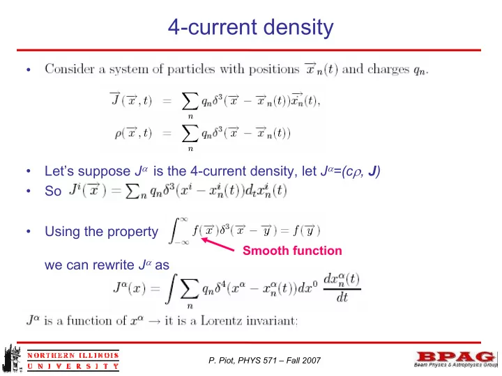
4-current density • …. Let’s suppose J α is the 4-current density, let J α =(c ρ , J ) • • So • Using the property Smooth function we can rewrite J α as P. Piot, PHYS 571 – Fall 2007

Charge continuity equation • Consider the divergence of J • So charge continuity can be written as P. Piot, PHYS 571 – Fall 2007

4-gradient • In previous slide we introduce the 4-gradient operator • This operator transforms as • Note that • Can define the covariant form • The self-contraction yields the d’Alembertian: P. Piot, PHYS 571 – Fall 2007

4-potential • Define • This is precisely the equation we solved to get the field of a moving charge three lessons ago… In SI unit : φ → c φ • • In SI unit P. Piot, PHYS 571 – Fall 2007

Covariance of Maxwell equations • Define the tensor of dimension 2 4 potential 4 potential • F , is the e.m. field tensor. It is easily found to be In SI units, F is obtained by E → E/c • • The covariant form is P. Piot, PHYS 571 – Fall 2007

Inhomogeneous Maxwell’s eqns • Consider • Similarly • The inhomogeneous Maxwell’s equations can be caster under the equation P. Piot, PHYS 571 – Fall 2007

Homogeneous Maxwell’s eqns I • Consider the Levi-Civita tensor (rank 4) • And consider P. Piot, PHYS 571 – Fall 2007

Homogeneous Maxwell’s eqns II • Consider the Levi-Civita tensor (rank 4) • The homogeneous Maxwell’s equations can be caster under the equation With the Dual field tensor defined as P. Piot, PHYS 571 – Fall 2007

Covariant form of Maxwell’s equation • To introduce H and D field introduce the rank 2 tensor: • Then Maxwell’s equation writes • F is a rank 2 tensor that conforms to Lorentz transformation so the (E,B) field can be computed in an other frame by or, in matrix notation P. Piot, PHYS 571 – Fall 2007

Covariant form of Maxwell’s equation • Example consider the Lorentz boost along z- axis • Then from • We get the same matrix as [JDJ 11.148] P. Piot, PHYS 571 – Fall 2007

Invariant of the e.m. field tensor • Consider the following invariant quantities • Usually one redefine these invariants as • Which can be rewritten as where • Finally note the identities P. Piot, PHYS 571 – Fall 2007

Eigenvalues of the e.m. field tensor • The eigenvalues are given by • Characteristic polynomial • With solutions P. Piot, PHYS 571 – Fall 2007

Equation of motion • The equation of motion (EOM) can be written where • This is equivalent to defining a 4-force: • We need to solve EOM once we have specified the external e.m. tensor (assuming no other fields) P. Piot, PHYS 571 – Fall 2007