3D Vision: Multi-View Stereo & Volumetric Modeling Torsten - PowerPoint PPT Presentation
3D Vision: Multi-View Stereo & Volumetric Modeling Torsten Sattler, Martin Oswald Spring 2018 http://www.cvg.ethz.ch/teaching/3dvision/ Schedule Feb 19 Introduction Feb 26 Geometry, Camera Model, Calibration Mar 5 Features, Tracking
3D Vision: Multi-View Stereo & Volumetric Modeling Torsten Sattler, Martin Oswald Spring 2018 http://www.cvg.ethz.ch/teaching/3dvision/
Schedule Feb 19 Introduction Feb 26 Geometry, Camera Model, Calibration Mar 5 Features, Tracking / Matching Mar 12 Project Proposals by Students Mar 19 Structure from Motion (SfM) + papers Mar 26 Dense Correspondence (stereo / optical flow) + papers Apr 2 Bundle Adjustment & SLAM + papers Apr 9 Student Midterm Presentations Arp16 Easter break Apr 23 Multi-View Stereo & Volumetric Modeling + papers Whitsundite Apr 30 May 7 3D Modeling with Depth Sensors + papers May 14 3D Scene Understanding + papers May 21 4D Video & Dynamic Scenes + papers May 28 Student Project Demo Day = Final Presentations 2
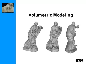
Multi-View Stereo & Volumetric Modeling 3
Motivation: Multi-view 3D reconstruction is hard! 4
Motivation: Multi-view 3D reconstruction is hard! 5
Motivation: Multi-view 3D reconstruction is hard! 6
Today’s class Modeling 3D surfaces by means of volumetric representations (implicit surfaces). In particular: • Surface representations • Extracting a triangular mesh from an implicit voxel grid representation (Marching Cubes) • Convex 3D shape modeling on a regular voxel grid • Building a triangular mesh from a non-regular volumetric grid 7
Surface Representations explicit / surface implicit / volumetric • Point cloud • Voxel grid • Occupancy grid • Spline / • Signed-distance NURBS grid • Voxel octree • Surface Mesh • Tetrahedral Mesh 8
Volumetric Representation • Voxel grid : sample a volume containing the surface of interest uniformly • Label each grid point as lying inside or outside the surface Signed distance function Occupancy function OF = 0.5 SDF = 0 OF = 0 SDF > 0 OF = 1 SDF < 0 • The modeled surface is represented as an isosurface (e.g. SDF = 0 or OF = 0.5) of the labeling (implicit) function 9
Volumetric Representation Why volumetric modeling? • Flexible and robust surface representation • Handles (changes of) complex surface topologies effortlessly • Ensures watertight surface / manifold / no self- intersections • Allows to sample the entire volume of interest by storing information about space opacity • Voxel processing is often easily parallelizable Drawbacks: • Requires large amount of memory (+processing time) • Scales badly to large scenes (cubic growth for voxels) 10
From volume to mesh: Marching Cubes “Marching Cubes: A High Resolution 3D Surface Construction Algorithm”, William E. Lorensen and Harvey E. Cline, Computer Graphics (Proceedings of SIGGRAPH '87). • March through the volume and process each voxel: • Determine all potential intersection points of its edges with the desired iso-surface • Precise localization of intersections via interpolation • Intersection points serve as vertices of triangles: • Connect vertices to obtain triangle mesh for the iso- surface • Can be done per voxel 11
From volume to mesh: Marching Cubes Example: “Marching Squares” in 2D 12
From volume to mesh: Marching Cubes By summarizing symmetric configurations, all possible 2 " = 256 cases reduce to: 13
From volume to mesh: Marching Cubes • The accuracy of the computed surface depends on the volume resolution • Precise normal specification at each vertex possible by means of the implicit function (via gradient) 14
From volume to mesh: Marching Cubes • Benefits of Marching Cubes: • Always generates a manifold surface • The desired sampling density can easily be controlled • Trivial merging or overlapping of different surfaces based on the corresponding implicit functions: • minimum of the values for merging • averaging for overlapping 15
From volume to mesh: Marching Cubes • Limitations of Marching Cubes • Maintains 3D entries rather than a 2D surface, i.e., higher computational and memory requirements • Generates consistent topology, but not always the topology you wanted • Problems with very thin surfaces if resolution not high enough 16
Convex 3D Modeling “Continuous Global Optimization in Multiview 3D Reconstruction”, Kalin Kolev, Maria Klodt, Thomas Brox and Daniel Cremers, International Journal of Computer Vision (IJCV ‘09). • Multiview stereo allows to compute entities of the type: ρ ∶ 𝑊 → [0,1] photoconsistency map reflecting the • agreement of corresponding image projections • 𝑔 ∶ 𝑊 → [0,1] potential function representing the costs for a voxel for lying inside or outside the surface • How can these measures be integrated in a consistent and robust manner? 17
Convex 3D Modeling • Photoconsistency usually computed by matching image projections between different views • Instead of comparing only the pixel colors, image patches are considered around each point to reach better robustness • Challenges: • Many real-world objects do not satisfy the underlying Lambertian assumption • Matching is ill-posed, as there are usually a lot of different potential matches among multiple views • Handling visibility 18
Convex 3D Modeling • A potential function can be obtained by f : V → [0 , 1] fusing multiple depth maps or with a direct 3D approach • Depth map estimation fast but errors might propagate during two-step method (estimation & fusion) • Direct approaches generally computationally more intense but more robust and flexible (occlusion handling, projective patch distortion etc.) 19
Convex 3D Modeling convex hull silhouette • Standard approach for potential function : f : V → [0 , 1] silhouette- / visual hull-based constraints • Problems with concavities • Propagation scheme handles concavities • Additional advantage: Voting for position with best photoconsistency defines denoised map ρ 20
Convex 3D Modeling Example: Middlebury “dino” data set standard silhoutte denoised stereo-based ρ f 21
Convex 3D Modeling • 3D modeling problem as energy minimization over volume V : • Indicator function for interior: • Minimization over set of possible labels: • Above function convex, but domain is not • Constrained convex optimization problem by relaxation to • Global minimum of E over C bin can be obtained by minimizing over C rel and thresholding solution at some 22
Convex 3D Modeling • Properties of Total Variation (TV) • Preserves edges and discontinuities: • coarea formula: 23
Convex 3D Modeling input images (2/28) input images (2/38) 24
Convex 3D Modeling • Benefits of the model • High-quality 3D reconstructions of sufficiently textured objects possible • Allows global optimization of problem due to convex formulation • Simple construction without multiple processing stages and heuristic parameters • Computational time depends only on the volume resolution and not on the resolution of the input images • Perfectly parallelizable 25
Convex 3D Modeling • Limitations of the model: • Computationally intense (depending on volume resolution): Can easily take up 2h or more on single- core CPU • Need additional constraints to avoid empty surface • Tendency to remove thin surfaces • Problems with objects strongly violating Lambertian surface assumption: Potential function might be f inaccurate 26
Convex 3D Modeling “Integration of Multiview Stereo and Silhouettes via Convex Functionals on Convex Domains”, Kalin Kolev and Daniel Cremers, European Conference on Computer Vision (ECCV ‘08). • Idea: Extract the silhouettes of the imaged object and use them as constraints to restrict the domain of feasible shapes 27
Convex 3D Modeling • Leads to the following energy functional: • denotes silhouette in image i Sil i ⊂ Ω i • denotes ray through pixel j in image i R ij • Solution can be obtained via relaxation and subsequent thresholding of result with appropriate threshold 28
Convex 3D Modeling input images (2/24) input images (2/27) 29
Convex 3D Modeling • Benefits of the model • Allows to impose exact silhouette consistency • Highly effective in suppressing noise due to the underlying weighted minimal surface model • Limitations of the model • Presumes precise object silhouettes which are not always easy to obtain • The utilized minimal surface model entails a shrinking bias, tends to oversmooth surface details 30
Convex 3D Modeling “Anisotropic Minimal Surfaces Integrating Photoconsistency and Normal Information for Multiview Stereo”, Kalin Kolev, Thomas Pock and Daniel Cremers, European Conference on Computer Vision (ECCV ‘10). • Idea: Exploit additionally surface normal information to counteract the shrinking bias of the weighted minimal surface model 31
Convex 3D Modeling • Generalization of previous energy functional: • Matrix mapping defined as • is the given normal field • Parameter reflects confidence in the surface normals 32
Convex 3D Modeling input images (4/21) 33
Recommend
More recommend
Explore More Topics
Stay informed with curated content and fresh updates.
