
SLIDE 1
3D convection, phase change, and solute transport in mushy sea ice
Dan Martin, James Parkinson, Andrew Wells, Richard Katz
Lawrence Berkeley National Laboratory (USA), Oxford University (UK).
Summary:
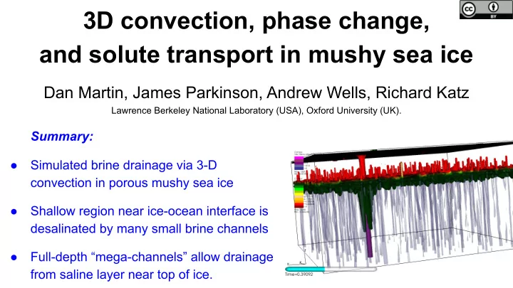
- Simulated brine drainage via 3-D
convection in porous mushy sea ice
- Shallow region near ice-ocean interface is
desalinated by many small brine channels
- Full-depth “mega-channels” allow drainage