3 2 1 Resource dep. 0 0.5 1 2 3 (b) (c) With bad - - PowerPoint PPT Presentation

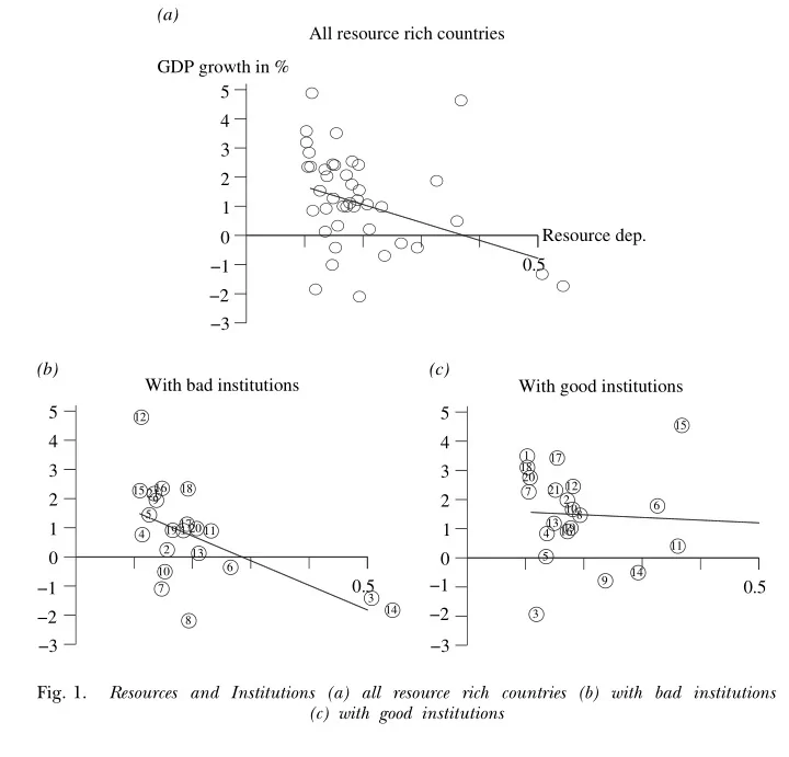
0.5 −3 −2 −1 1 2 3 4 5 GDP growth in % Resource dep. All resource rich countries (a) 0.5 −3 −2 −1 1 2 3 4 5

2 3 4 6 7 8 9 5 10 11 12 13 14 15 16 17 18 19 20 21

.

With bad institutions (b) 0.5 −3 −2 −1 1 2 3 4 5

1 2 3 4 5 6 7 8 9 10 11 12 13 14 15 16 17 18 19 20 21

With good institutions (c)

• Fig. 1.

Resources and Institutions (a) all resource rich countries (b) with bad institutions (c) with good institutions

Table 1 Regression Results I

Dependent variable: GDP growth. Regression 1 Regression 2 Regression 3 Regression 4 Initial income level 0.79* 1.02* 1.28* 1.26* (3.80) (4.38) (6.65) (6.70) Openness 3.06* 2.49* 1.45* 1.66* (7.23) (4.99) (3.36) (3.87) Resource abundance 6.16* 5.74* 6.69* 14.34* (4.02) (3.78) (5.43) (4.21) Institutional quality 2.2* 0.6 1.3 (2.04) (0.64) (1.13) Investments 0.15* 0.16* (6.73) (7.15) Interaction term 15.4* (2.40) Observations 87 87 87 87 Adjusted R2 0.50 0.52 0.69 0.71 Note: The numbers in brackets are t-values. A star (*) indicates that the estimate is significant at the 5-% level.

Table 2 Regression Results II

Dependent variable: GDP growth. Regression 1 Regression 2 Regression 3 Regression 4 Regression 5 Regression 6 Initial income level 1.33* 1.88* 1.33* 1.34* 1.36* 1.45* (6.26) (7.95) (5.90) (6.97) (6.13) (5.45) Openness 1.87* 1.34* 1.60* 1.59* 1.63* 1.56* (3.77) (3.20) (3.47) (3.73) (3.76) (3.36) Resource abundance 10.92* 16.35* 13.70* 14.78* 16.25* (3.16) (3.71) (4.00) (4.26) (3.60) Mineral abundance 17.71* (3.16) Institutional quality 0.20 1.83 0.90 1.15 1.18 0.78 (0.22) (1.35) (0.69) (0.96) (0.94) (0.56) Investments 0.15* 0.11* 0.15* 0.15* 0.15* 0.14* (6.25) (4.09) (5.56) (6.51) (6.76) (4.91) Interaction term 29.43* 11.01 18.31* 15.86* 16.84* 19.01* (2.66) (1.84) (2.34) (2.45) (2.55) (2.41) Secondary 0.60 0.57 (0.44) (0.41) Ethnic frac. 0.88 0.77 (1.69) (1.12) Language frac. 0.36 0.11* (0.75) (0.18) Africa exluded no yes no no no no Observations 87 59 76 86 84 74 Adjusted R2 0.63 0.79 0.70 0.71 0.70 0.70 Note: The numbers in brackets are t-values. A star (*) indicates that the estimate is significant at the 5-% level.

| | | | | | | | | | | | | | | | | | | | | | | | | | | | | | | | | | | | | | | | | | | | | | | | | | | | | | | | | | | | | | | | | | | | | | | | | | | | | | | | | | | | | |

−20 −10 10 20 Effect of resources on growth 5 10 Institutional quality

Table 2: Conflicts and mineral prices

(1) (2) (3) (4) (5) (6) Estimator LPM

• Dep. var.

Conflict incidence Sample All V(Mkt) = 0 All V(Mkt) = 0 mine > 0 0.112c 0.048 (0.065) (0.065) ln price main mineral

• 0.029

0.028 (0.032) (0.019) ln price × mines > 0 0.086b 0.072a 0.060a 0.085a 0.108a (0.034) (0.020) (0.021) (0.024) (0.041) ln price × mines > 0 (neighbouring cells) 0.021a (0.006) ln price × mines > 0 (ever) 0.045a (0.014) Country×year FE Yes Yes Yes Yes No No Year FE No No No No Yes Yes Cell FE Yes Yes Yes Yes Yes No Neighborhood FE No No No No No Yes Observations 143768 142296 127974 143864 142296 17360

LPM estimations.

c significant at 10%; b significant at 5%; a significant at 1%.

Conley (1999) standard errors in parentheses, allowing for spatial correlation within a 500km radius and for infinite serial correlation. mine > 0 is a dummy taking the value 1 if at least 1 mine is active in the cell in year t. mines > 0 (ever) is a dummy taking the value 1 if at least 1 mine is recorded in the cell at any point over the 1997-2010

• period. mines > 0 (neighbouring cells) is a dummy taking the value 1 if at least 1 mine is recorded in neighbouring cells of degree 1 and 2

in year t. V(Mkt) = 0 means that we consider only cells in which the mine dummy (or dummies in column (3)) takes always the same value

• ver the period. Column (6) is estimated on a sample containing only mining cells and their immediate neighboring cells. In columns (1) to

(5), ln price main mineral is the World price of the mineral with the highest production over the period (evaluated at 1997 prices) for mining cells, and zero for non-mining cells. In column (6) ln price main mineral takes the same value for the mining cell and its immediate neighbours. Estimations (1) and (6) include controls for the average level of mineral World price interacted with the mine dummy.

Table 5: Minerals price and types of conflict events

(1) (2) (3) (4) (5) (6) LPM Sample V(Mkt) = 0 All V(Mkt) = 0 All V(Mkt) = 0 All Conflict incidence var. Battles Violence against civ. Riots / Protests ln price × mines > 0 0.016b 0.040a 0.044b (0.008) (0.014) (0.018) ln price × mines > 0 (ever) 0.002 0.034a 0.038a (0.006) (0.010) (0.011) Country×year FE Yes Yes Yes Yes Yes Yes Cell FE Yes Yes Yes Yes Yes Yes Observations 142296 143864 142296 143864 142296 143864

LPM estimations.

c significant at 10%; b significant at 5%; a significant at 1%.

Conley (1999) standard errors in parentheses, allowing for spatial correlation within a 500km radius and for infinite serial correlation. mine > 0 is a dummy taking the value 1 if at least 1 mine is active in the cell in year t. mines > 0 (ever) is a dummy taking the value 1 if at least 1 mine is recorded in the cell at any point over the 1997-2010

• period. V(Mkt) = 0 means that we consider only cells in which the mine dummy takes always the same value over the period. ln price main

mineral is the World price of the mineral with the highest production over the period (evaluated at 1997 prices) for mining cells, and zero for non-mining cells.